
This page derives from a presentation on The Objective Evaluation of Human Hearing in March 2019 at the meeting of the Deutsche Gesellschaft für Audiologie in Heidelberg. The notes for the presentation and the actual PowerPoint file are available to download. The sound samples are not directly accessible through this page but are available in the PowerPoint file. Some general references for this talk are Picton (2011) and Hoth et al. (2014).
I. Audiometry
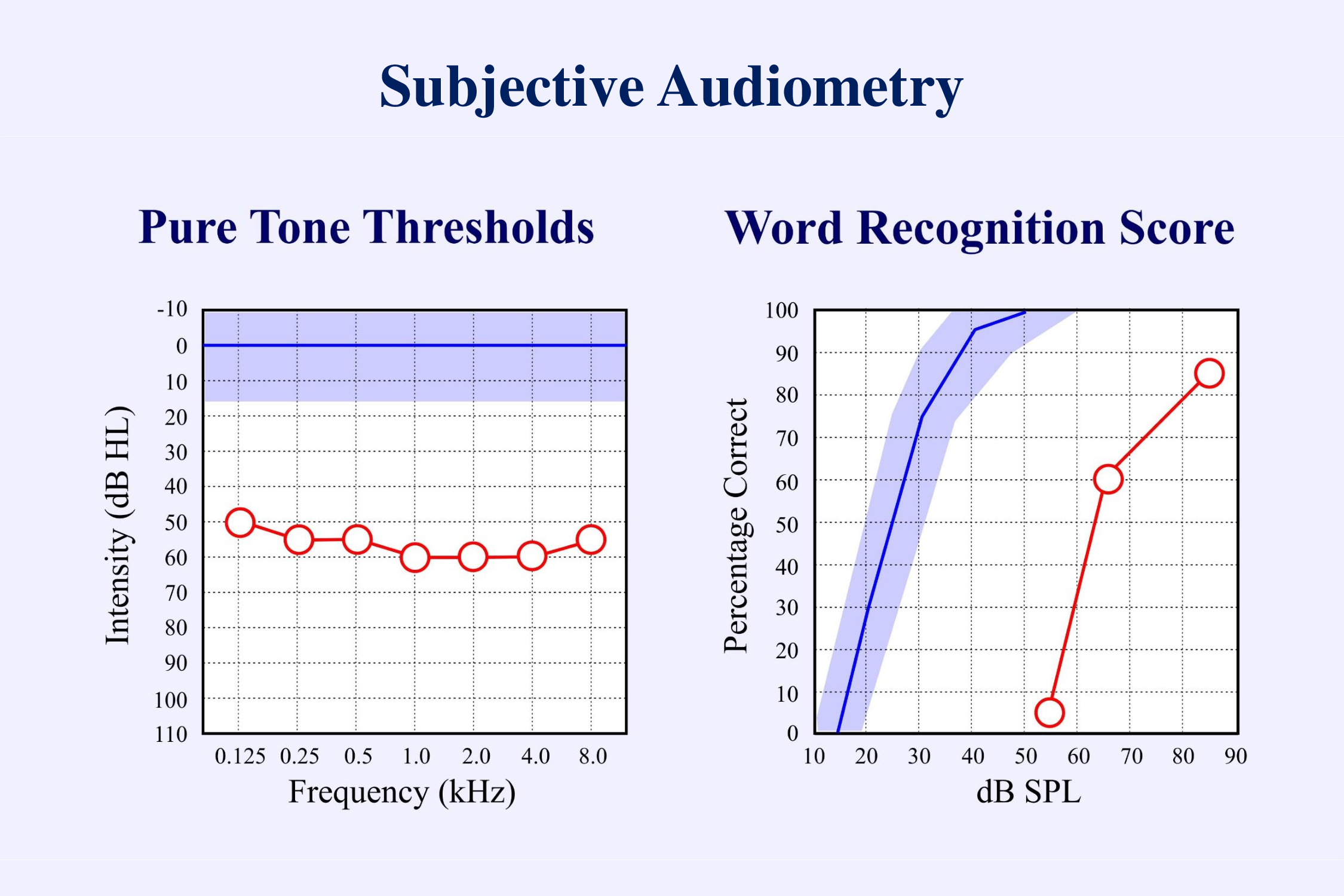
Subjective audiometry has two main parts: the pure tone audiogram and the word recognition score. Both are “subjective” in that they require the subject to make a conscious response – to press a button when a tone has been heard or to repeat a word that was just presented. We can often predict the word recognition score from the pure tone thresholds. This has led many to disregard the results of speech perception studies. Hearing aids are usually fit mainly on the basis of the pure tone audiogram. Speech perception is given little attention. One of the goals of this presentation is to promote the testing of speech.
a) Objective Audiometry
Subjective audiometry requires both a conscious response from the person being tested, and an interpretation of this response by the audiologist performing the test. “Objective” audiometry does not require a conscious response from the patient. I shall propose that fully objective audiometry should also not require any conscious interpretation of the results by the audiologist. Present techniques of objective audiometry can provide good estimates of the pure tone audiogram. However, there is as yet no objective measurement of speech perception.
Several objective responses to sound can be recorded without the subject having to make a decision and provide a behavioral response:
- changes in the heart rate
- reflex movements in the body
- middle ear muscle reflexes
- otoacoustic emissions
- electrical responses from the ear or brain
- magnetic responses from the brain
- changes in cerebral blood flow as measured with magnetic resonance imaging (fMRI) or event-related optical signals (near-infra-red spectroscopy NIRS)
I shall limit myself to the electrical measurements:
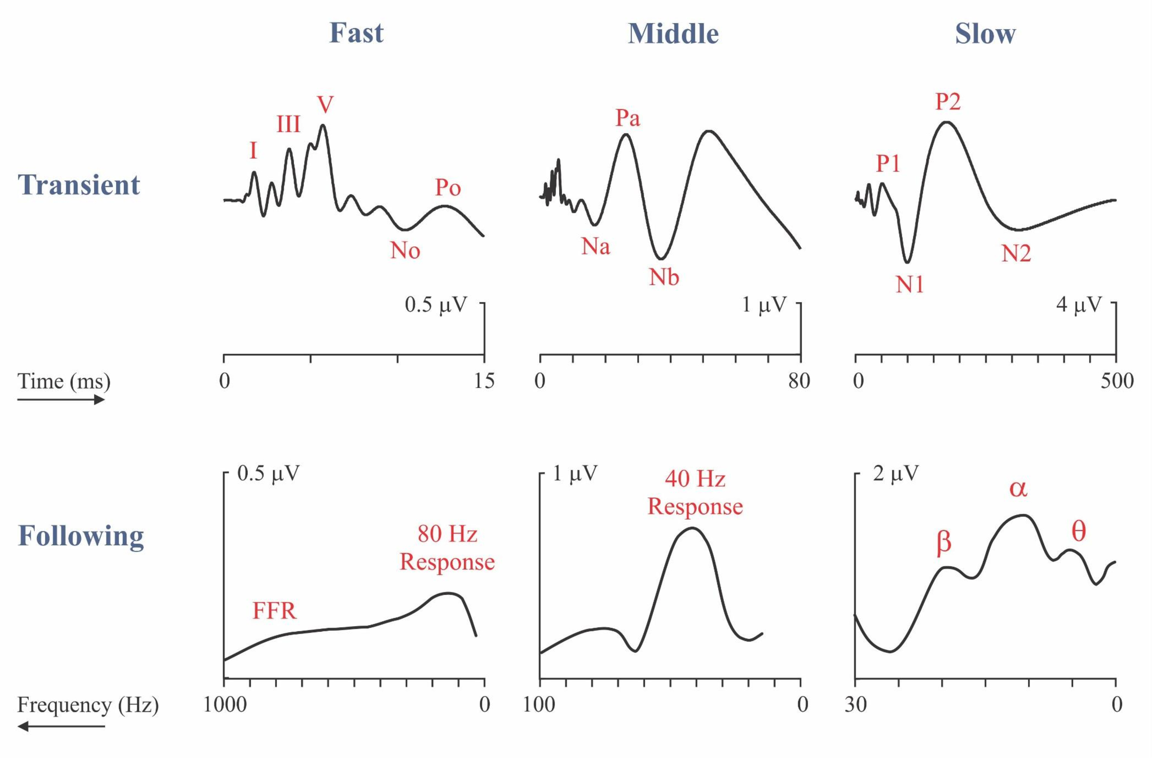
The illustration (Picton, 2013) shows the electrical responses to sound categorized as transient or following responses. The upper half of the figure shows the transient auditory evoked potentials plotted on three different time scales – fast, middle and slow. The waveforms represent the typical response to 70 dB nHL clicks presented at a rate of 1/s. The lower half of the figure represents the following responses recorded to amplitude-modulated noise presented at 60 dB SPL when the rate of modulation is varied. These following responses are plotted on three different frequency scales with the slower responses on the right. Though initially counter-intuitive, this arrangement of the axis allows comparison between homologous transient and following responses. The peaks of the slow following responses near 4, 10 and 20 Hz have been named θ, α, and β after the frequency-bands of the human EEG. Until recently most of the studies of the auditory following responses concentrated on the 40 Hz response (also known as the γ response), the 80 Hz response and the fast Frequency Following Response. Recently the slow following response (labelled θ) has be shown to be important in following the speech envelope.
Objective hearing tests are useful in many situations:
- subjects too young to provide reliable behavioral responses.
- patients who are too emotionally disturbed or cognitively impaired to provide reliable behavioral responses.
- unconscious or anesthetized patients
- patients who may be consciously or unconsciously exaggerating their hearing impairment.
- evaluating patients with auditory neuropathy or auditory processing disorders.
- assessing the function of cochlear implants
The most important of these applications, and the one I shall focus on, is the evaluation of hearing in infants and young children. Different countries have different procedures for screening and diagnosis in the newborn period. This slide shows typical protocols:

Well babies are screened using otoacoustic emissions. Because of the possibility of auditory neuropathy, babies in an intensive care unit are screened using auditory brainstem responses (ABRs). Babies who fail the screening tests or who may have developed hearing loss after birth are referred for diagnostic evaluation – the estimation of thresholds at different frequencies. The usual approach records auditory brainstem responses to brief tones, or more recently to narrowband chirps.
b) Chirps
The major change in objective audiometry in the last decade has been the use of chirps. CE chirps designed by Claus Elberling are constructed to compensate for the frequency-related delays that occur in the cochlea (Elberling & Don, 2010; Elberling & Crone-Esmann, 2017; Gøtsche-Rasmussen et al., 2012). The travelling wave distributes the different frequencies of sound along the basilar membrane with the high frequencies near the stapes occurring a few milliseconds before the low frequencies near the apex. Chirps can be broad-band (like a click) or limited to an octave of frequencies (like a brief tone).
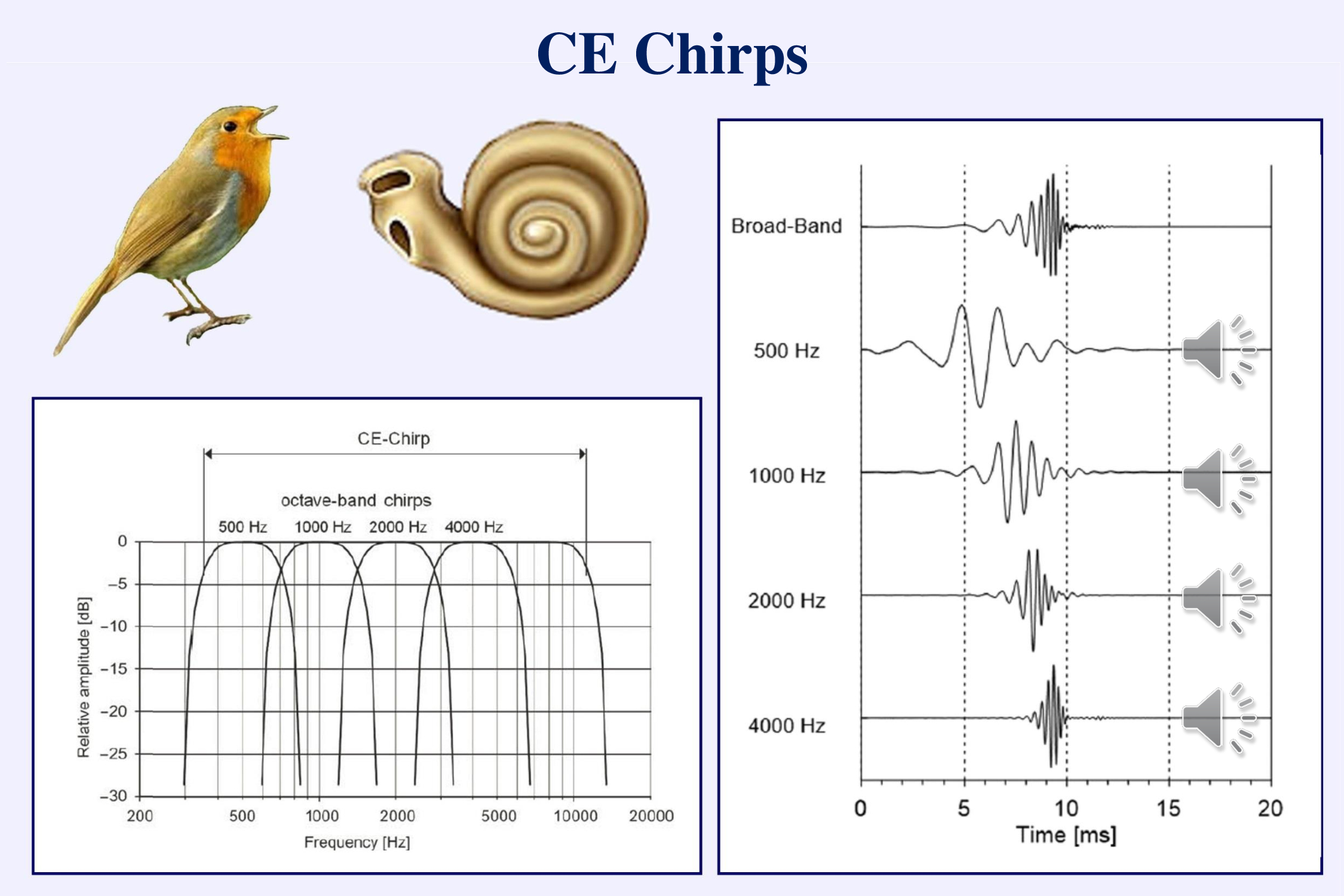
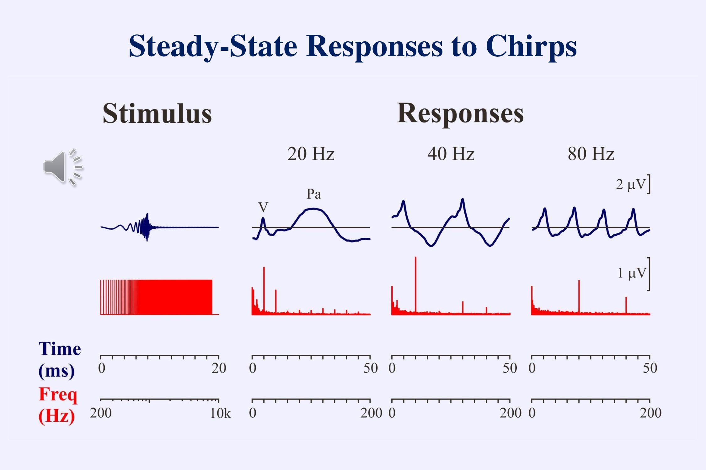
A transient stimulus contains multiple different frequencies. If the timings of these different frequencies are adjusted so that the slower frequencies begin earlier than the faster frequencies, the neural responses will all occur simultaneously rather than sequentially and the combined response will be larger. Larger responses shorten the time to recognize whether a response is present or not.

Tonepips and narrow-band chirps sound similar and have a similar acoustic specificity. However, as the preceding slide shows, the ABR evoked by a chirp is significantly larger than that evoked by a simple tonepip. In general, the wave V amplitude is about 50% larger when using chirps. This makes it faster to determine whether a response is present (Cobb & Stuart, 2016abc; Ferm et al., 2013; Ferm et al., 2015, Rodrigues et al., 2013).
A differently designed low-frequency chirp might provide more accurate assessment of low-frequency hearing, particularly if used with masking (Baljić et al., 2017; Frank et al., 2017), but this stimulus is not widely available:
c) Speech Perception
In order to facilitate the development of speech and language, once a baby has been identified as hearing-impaired, a full audiological evaluation must be performed and treatment initiated (Scollie & Bagatto, 2010).
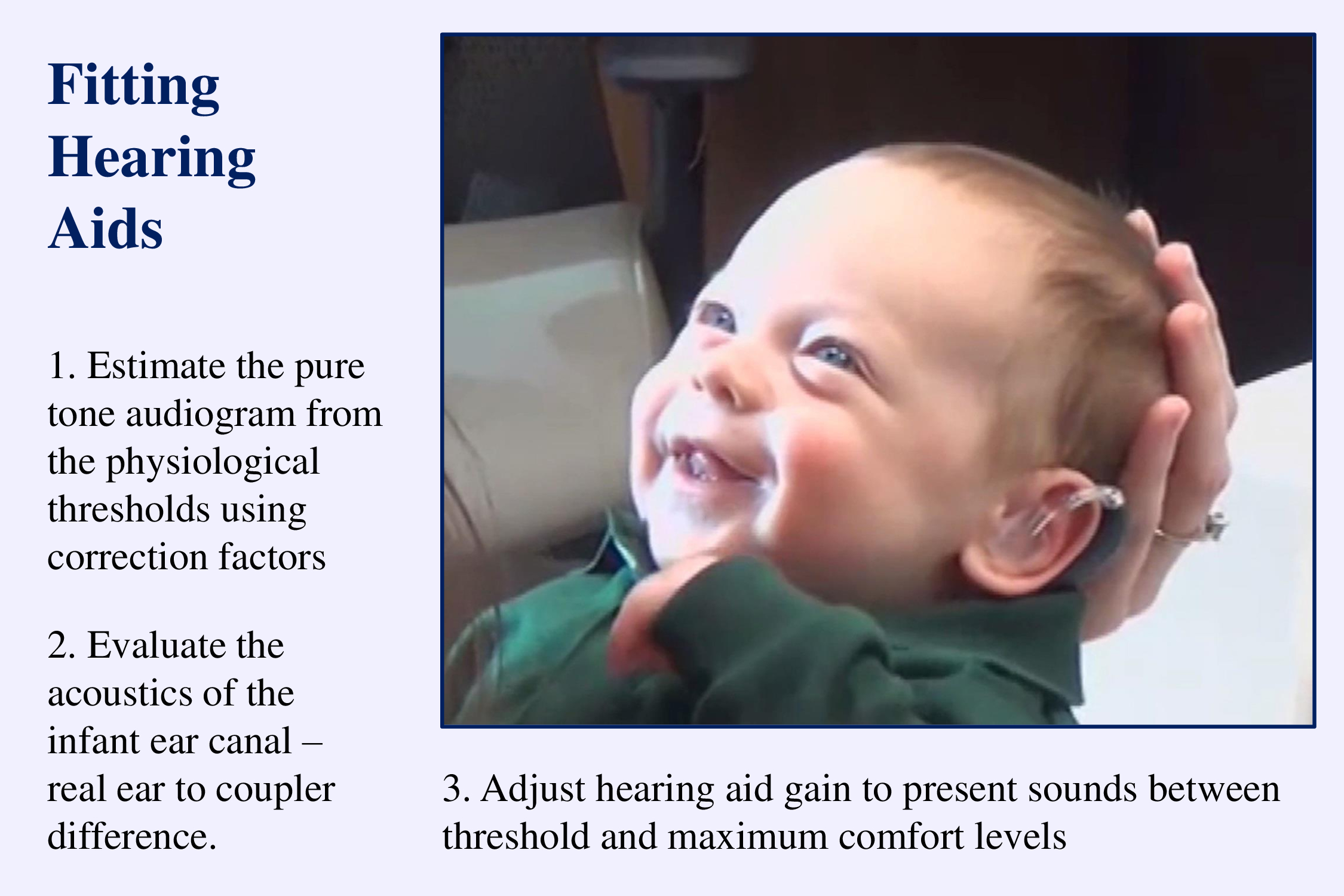
These procedures work well to provide the baby with amplified sounds. However, they do not guarantee that such sounds can be discriminated one from another or that they are perceived as speech. Even when fitting hearing aids in adults, one usually does not assess how well speech is perceived through the aids. One simply assumes that the amplified sound is adequate for communication. The problem is that the measurement of speech perception is time-consuming even when behavioral methods are used.
This is unfortunate. Patients come to the audiologist because they cannot understand speech. They do not usually complain of difficulties in hearing faint tones. We need to pay more attention to speech perception.
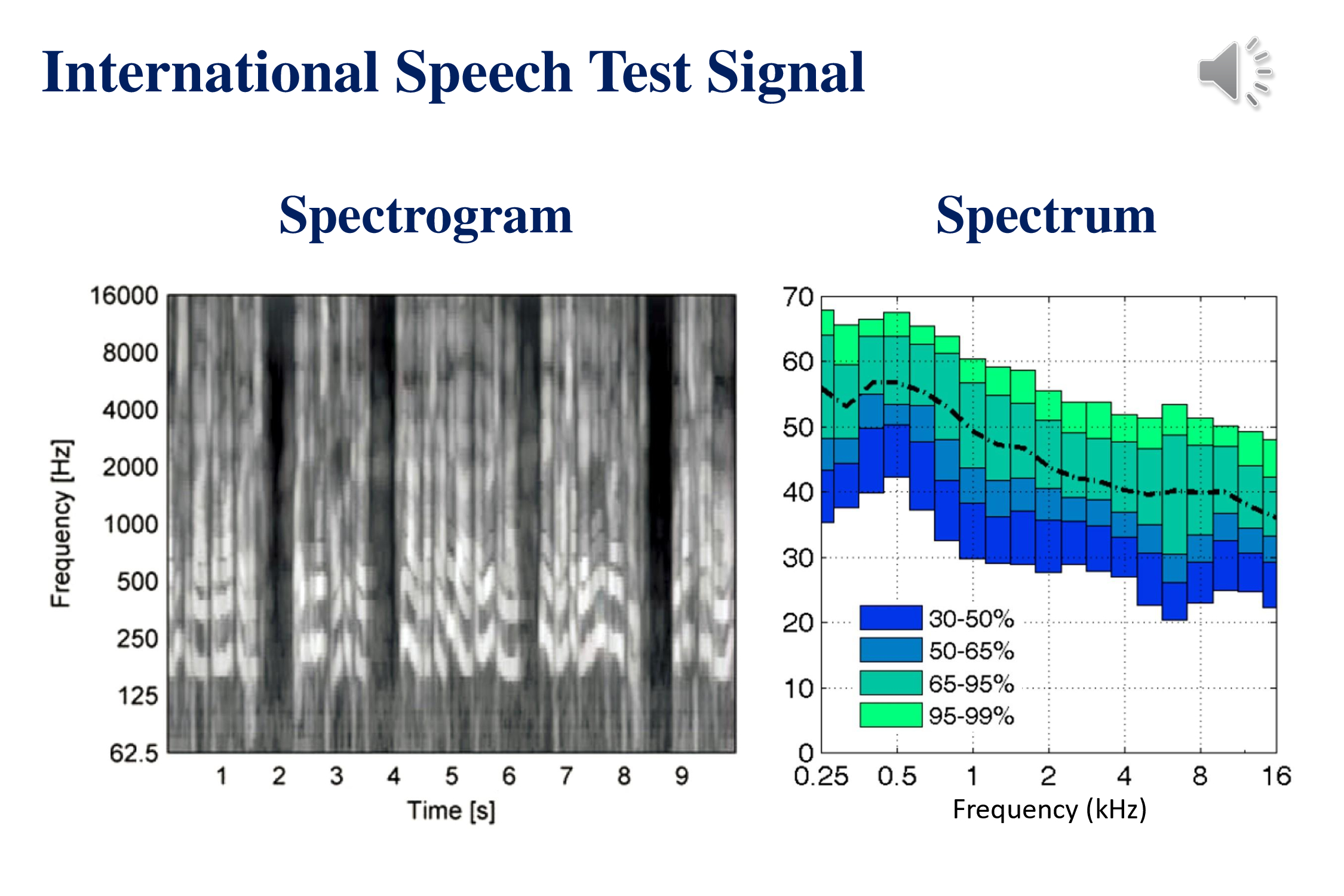
This slide shows the acoustic characteristics of the recently developed International Speech Test Signal (Holube et al., 2010). This was constructed by piecing together snippets of speech in 6 different languages: English, Arabic, Chinese, French, German and Spanish. The signal does not make any sense. Played in an endless loop it is a good cure for insomnia or a demonstration of how speech sounds when one is aphasic. The ISTS signal and supporting documents are available at the website of the European Hearing Instrument Manufacturers Association.
The spectrogram (left) demonstrates some of the temporal characteristics of speech – phonemes that last between tens of milliseconds, syllables that recur a rate of 3-5 per second, words that last around a second and phrases that last several seconds. The average speech spectrum (right) shows that most of the energy of speech is in the lower frequencies (Byrne et al., 1994). Not clear from these acoustic characteristics is the fact that many of the acoustic features that distinguish phonemes involve the middle and high frequencies.
Response to tones and chirps can tell us about hearing thresholds but they do not tell us whether the subject can perceive speech. How might we determine objectively whether a patient can discriminate between different sounds? We need to show that the brain can discriminate changes in the auditory stimulus:
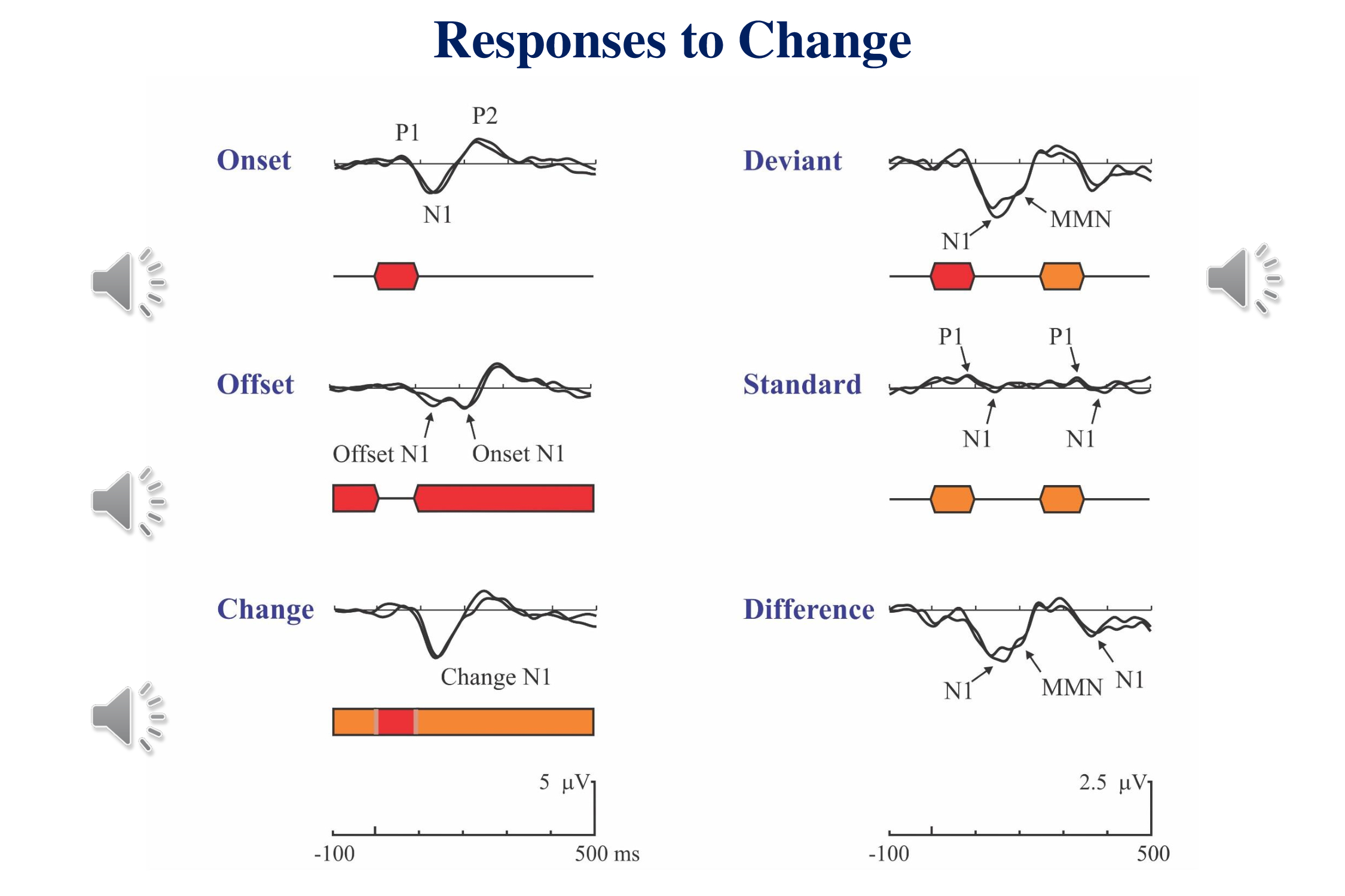
This slide (Figure 11-2 in Picton, 2011) shows the human cortical response to an auditory stimulus in different contexts. An occasional stimulus evokes a P1-N1-P2 complex. An occasional pause in an ongoing tone evokes a response to both the offset of the tone and its re-onset. A brief change in the frequency of a continuous tone evokes a similar response to the onset of a brief tone. These are simple responses to simple changes.
Things get more complicated when multiple stimuli are involved (right side of figure). If an occasional tone differs from the preceding tones, we record both a response to the onset and a later negative wave in response to the stimulus deviance – the mismatch negativity. The difference between this response and the response to an ongoing standard stimulus shows both the N1 of the onset-response and the MMN to the change. Also visible in these results is the fact that at rapid rates the N1 response to the standard is small whereas the P1 persists. As well as the N1 response to a standard being smaller than the response to the deviant, and the response to the standard that follows the deviant is larger than to a standard that follows another standard. The illustration is from
The mismatch negativity (MMN) does not require any subjective response on the part of the subject. The subject does not even have to attend to the stimuli. Furthermore the MMN can be recorded in response to phonetic changes as well as simple acoustic changes. The major problem with using the MMN as an objective test is that it is small and takes a long time to record.

A Mismatch Response can be recorded in response to a change in the phonetic characteristic of a stimulus. This slide from Angela Friederici et al. (2002) shows the response of young infants to a change in phoneme duration. In German, the duration of a vowel is meaningful. The mismatch response in the awake infant is similar to that in adults – a small negative wave, the mismatch negativity (MMN). However, in the sleeping infant the response is quite different – a large positive wave rather than a small negative wave. In this slide (as opposed to most of the other slides in this presentation) negative is plotted upward. We who study evoked potentials have often been accused of not knowing which way is up.
Audiometry – Conclusions
Chirps are good.
We do not yet have an objective assessment of speech perception.
II. Multiplicity
Now that we have considered the need for objective audiometry we shall look at three different aspects of this process – the principle of multiplicity, methods for identifying thresholds, and evaluating speech perception.
The principle of multiplicity entails that
- we should record responses to multiple stimuli simultaneously, and
- we should record multiple different responses to these stimuli.
a) Multiple Simultaneous Stimuli to Assess Pure Tone Thresholds
Many years ago, Otavio Lins and I (Lins & Picton, 1994; Lins et al., 1996) showed that we could record brainstem responses to multiple amplitude-modulated tones presented simultaneously. An amplitude modulated tone evokes a steady state response at the frequency of the modulation. This can be identified as a peak in the spectra of the responses on the right of the figure. Steady-state responses were evoked by different tones, each modulated at a unique frequency Each response is recorded separately.
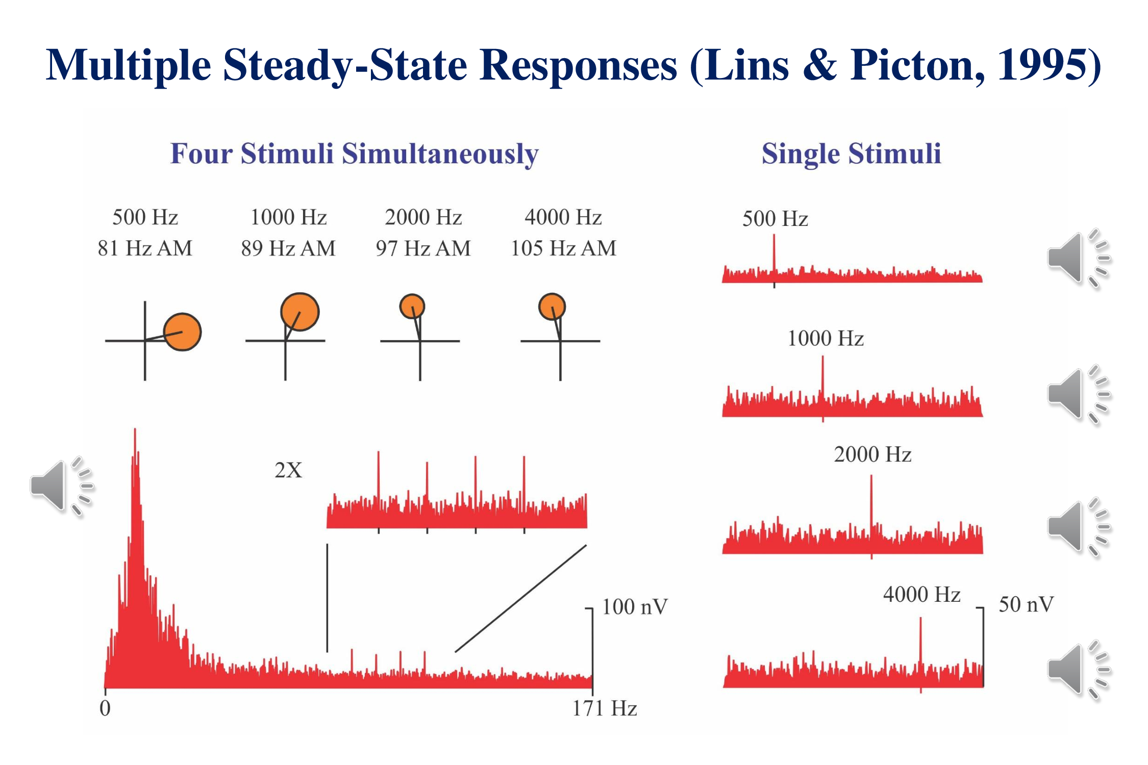
The left side of the figure shows what can be recorded when we combine the stimuli and present them simultaneously. If you pay attention to the sound you can recognize the individual stimuli in the mixture. The cochlea processes each of the modulated stimuli in a separate region of the basilar membrane.
The lower left shows the complete spectrum of the response to the combined stimuli. At the specific modulation-frequencies of each stimulus we can see a response. The region around these frequencies is amplified 2X in the inset. Each response can also be viewed on individual polar plots (upper left) which show the phase as well as the amplitude.
There is no difference in response-amplitude when the stimuli are presented simultaneously from when they stimuli are presented singly. It is therefore much more efficient to record the responses to multiple stimuli presented concurrently than to record each response separately. We can present four stimuli to the left ear and four stimuli to the right ear. In the best of all possible worlds we can get 8 thresholds in the same time that it takes to record one.
A major recent advance in the multiple stimulus technique has been to use chirps rather than amplitude modulated tones. The use of multiple chirp-trains instead of multiple amplitude modulated tone was initially proposed by Cebulla et al. (2012). These stimuli evoke larger responses and are more quickly detected. They can be recorded close to threshold in infants (upper right from Rodriguez et al., 2014) and the estimated thresholds correlate well with those obtained using simple tonepip-ABRs when each stimulus is presented singly (lower illustration from Sininger et al., 2018). Michel and Jørgensen (2017) have reported similar results.
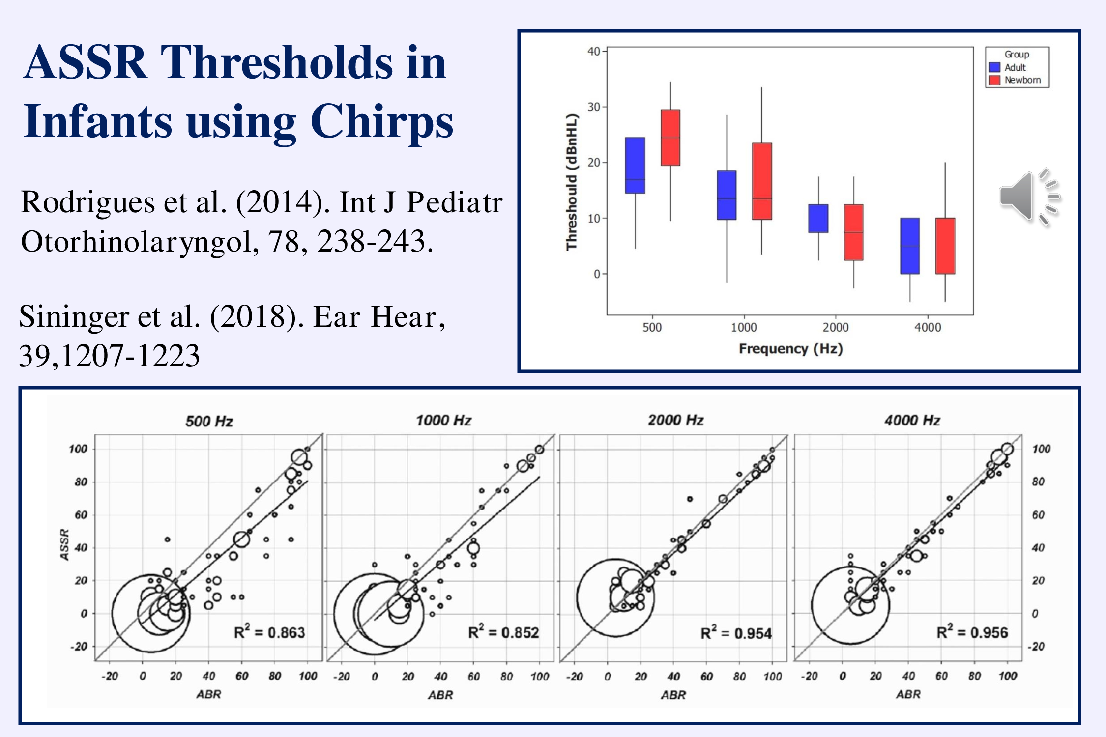
The advantage is that multiple chirp ASSRs over recording tone-pip ABRs is that the ASSRs can assess thresholds in much less time (20 as opposed to 32 minutes according to Sininger et al., 2018).
My recommendation for the objective determination of hearing thresholds is therefore to record the steady-state responses to multiple chirps presented simultaneously. This may best solve our need for estimating the pure tone audiogram. However it does not tell us that the subject can discriminate the sounds or perceive speech. Remember audiometry has two parts – pure tone thresholds and speech perception.
b) Multiple-Deviant Paradigm to Record Mismatch Responses
The idea of multiple simultaneous stimuli can be used to decrease the recording time for the mismatch negativity (MMN). The conventional MMN paradigm presents one type of deviant in a train of standards with a probability of 1/10. To record another type of MMN we need to repeat the whole recording. A “multiple-deviant” paradigm presents each deviant at the same temporal probability but presents five deviants – e.g., frequency, intensity, duration, frequency-glide and gap – concurrently (Näätänen et al., 2004).
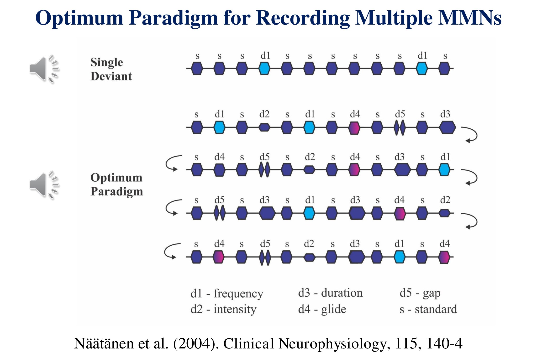
Five mismatch negativities for the price of one. The sound samples do not follow the illustration. Rather they give you a sense of what the stimuli sound like. We shall return to this paradigm later when we consider speech stimuli.
So now we have two protocols for presenting multiple stimuli simultaneously – auditory steady state responses to multiple chirps and mismatch responses to multiple deviances.
c) Multiple Responses
We should also consider the idea of recording multiple responses to the same stimuli. Where possible, we should record multiple responses – transient, sustained and steady-state – evoked by the same stimuli. The following illustration (Figure 10.12 of Picton, 2011) shows the responses to the intermittent amplitude modulation of a continuous tone – at 40 Hz and at 80 Hz. The modulations alternate in their phase. So averaging the responses to the different modulations together cancels out the steady-state response and leaves the transient and sustained potentials. The onset of the modulation evokes an onset response that consists mainly of a P1 wave. Since the stimuli are presented rapidly, the N1 is very small. A sustained potential lasts through the duration of the modulation.
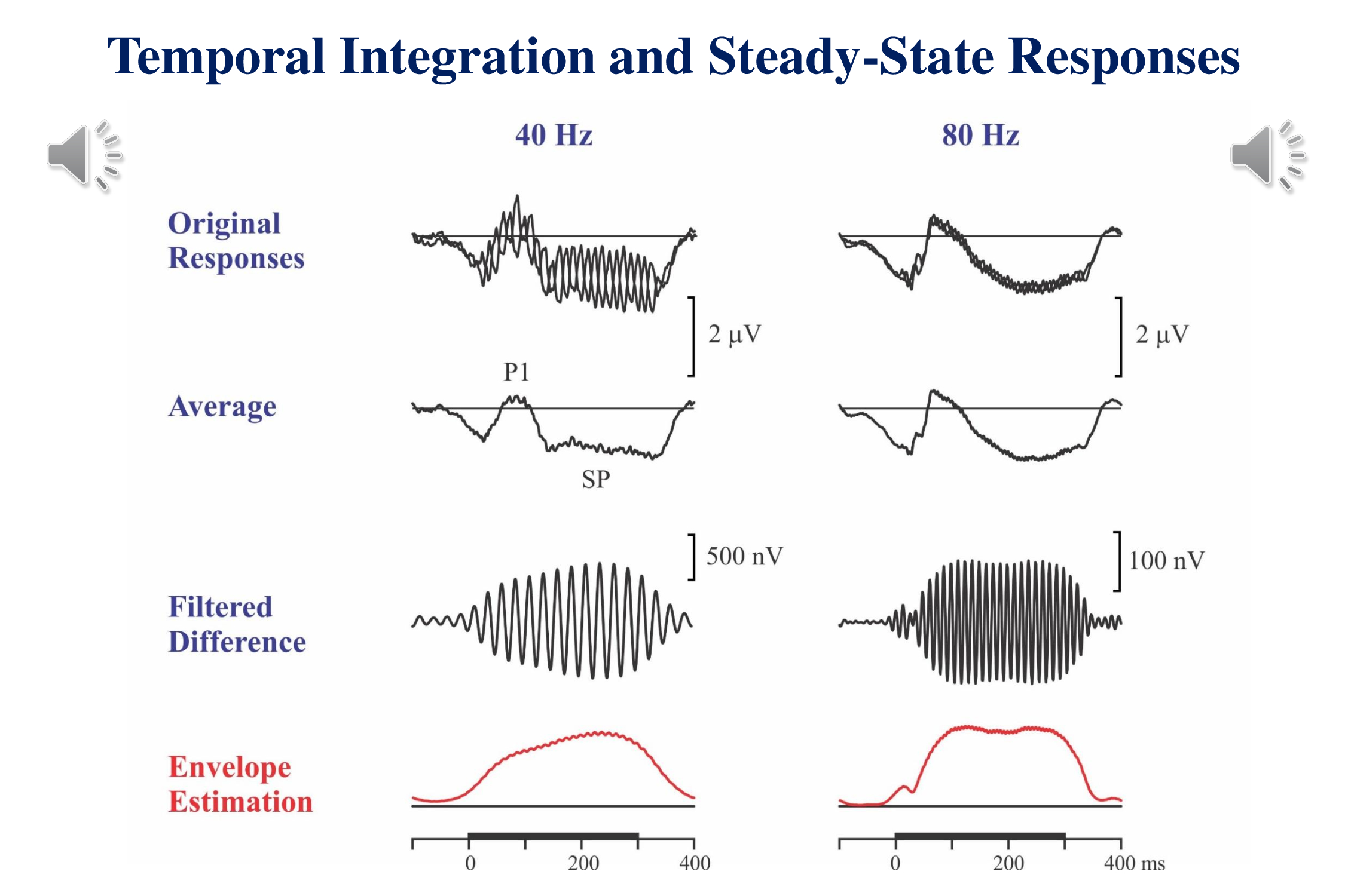
If we take the difference between the responses to the out-of-phase stimuli, we cancel the transient and sustained potentials and are left with the steady-state response – which can be filtered and amplified. These recordings show the build-up of the steady-state response over time. The 80 Hz response originating in the brainstem builds up quickly. There is a slight glitch in the buildup – probably related to the onset response to the start of the modulation. The cortical 40 Hz response takes about 200 ms to reach steady state.
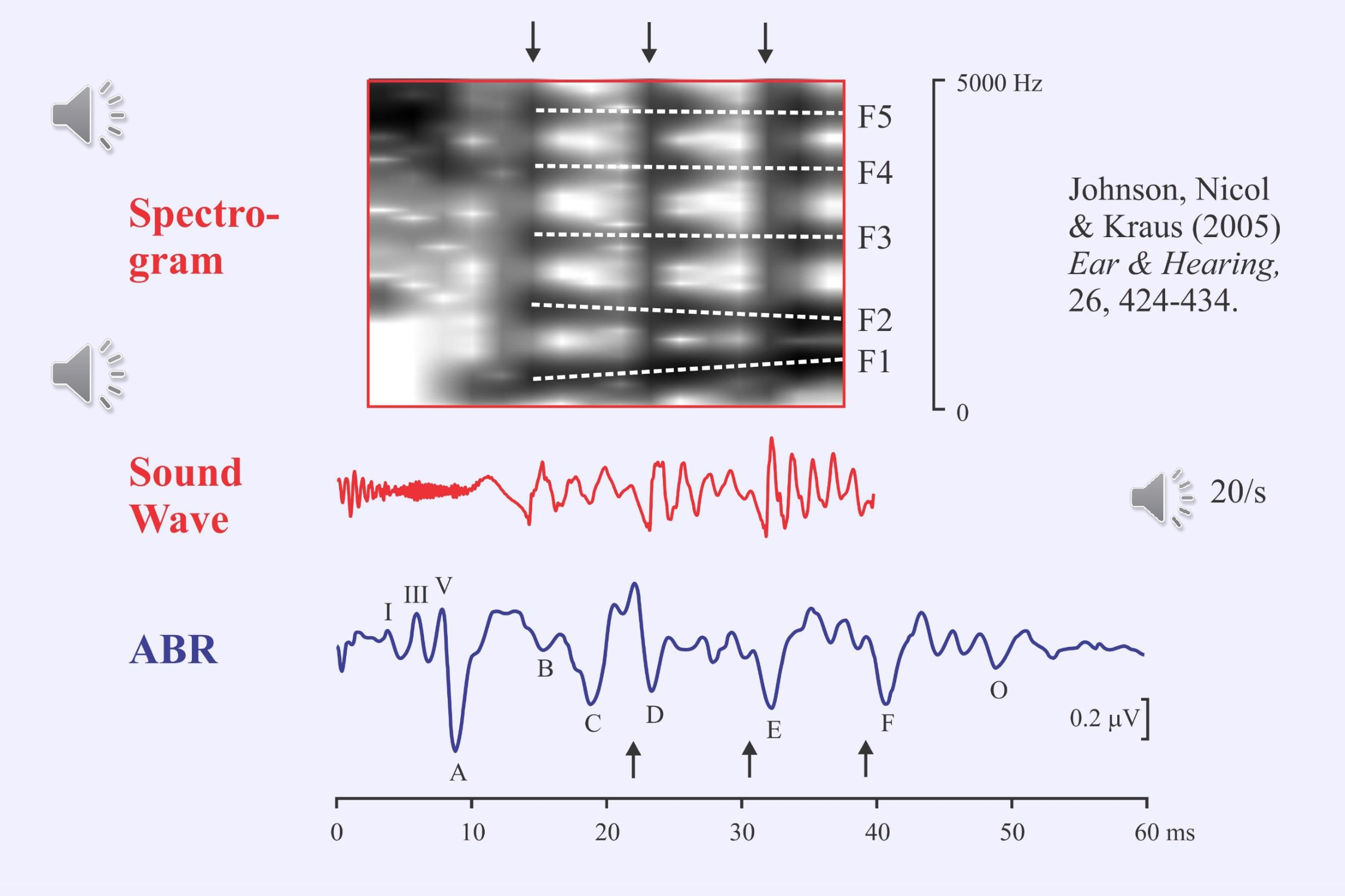
Frequency-following responses have long been evoked using pure tones. Nina Kraus and her colleagues have been using a special speech stimulus to evoke both transient and following responses (Johnson et al., 2005, 2008; Anderson et al., 2015; Bin Khamis et al., 2019). The syllable /da/ is truncated to just the first 40 ms and then repeated at 20/s. This stimulus elicits both the auditory brainstem response to the onset of the stop consonant and a frequency-following response to the beginning of the vowel. The large waves of the frequency-following response (D, E, F) occur about 7 ms after the onset of each of the glottal pulses. They represent the pitch envelope. The small waves in each glottal cycle represent the formant frequencies.
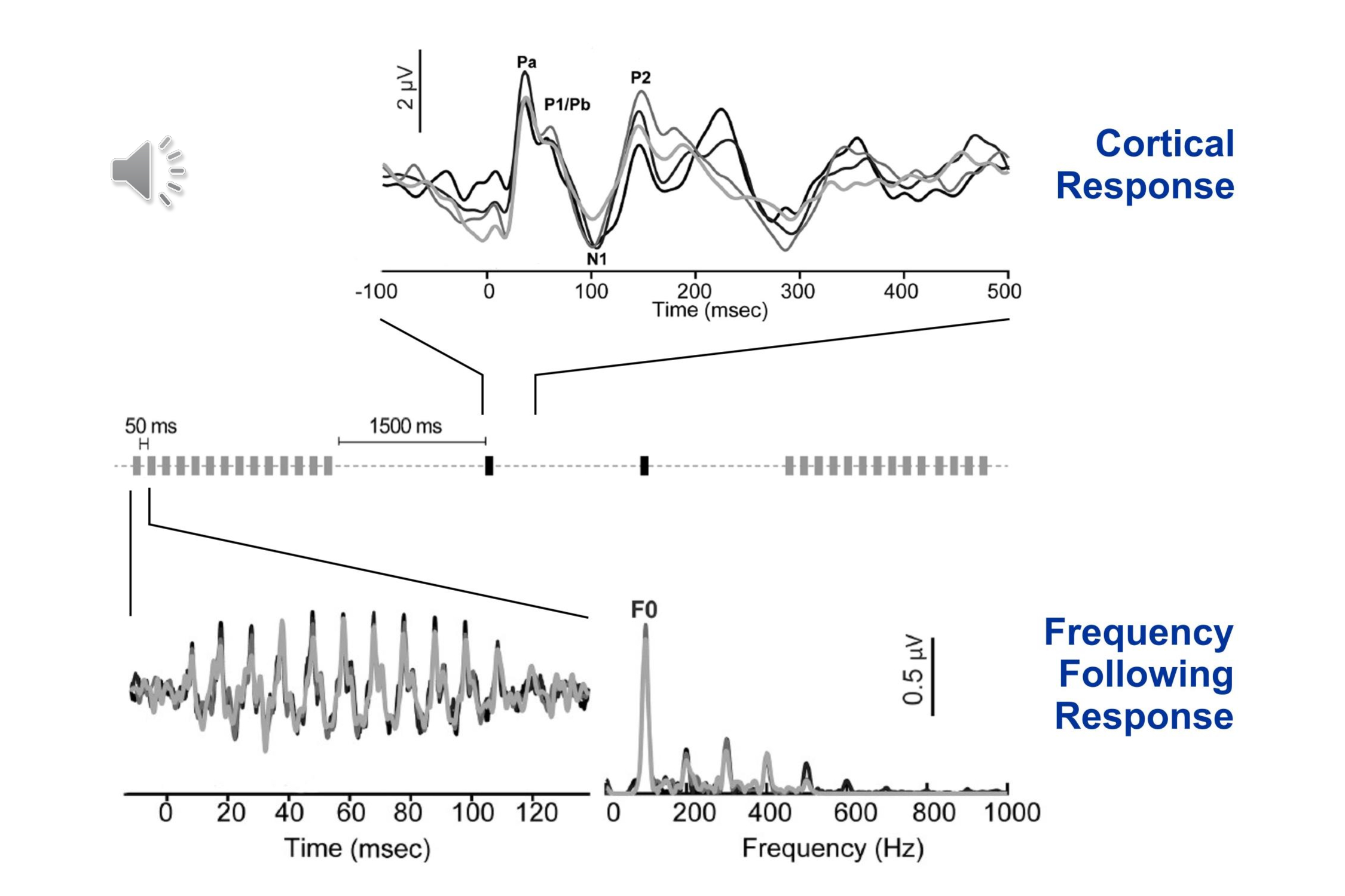
Another recently reported paradigm allows the recording of both the brainstem frequency following response and the cortical transient response (Bidelman, 2015; Bidelman et al., 2018). The stimulus is the vowel /a/. This is repeated rapidly to allow recording the brainstem frequency-following response, and then more slowly for recording the cortical onset response:
These last three illustrations are just examples. Where possible we should record multiple responses to the same stimuli. That way we might see how the sound is processed in different parts of the auditory system.
Conclusions – Multiplicity
The principle of multiplicity is established for the stimuli.
We still need to record multiple different responses to the same stimulus.
III. Threshold Detection
Objectivity means that the patient need not make a subjective response. Another aspect of objectivity involves the interpretation of the response and the determination of physiological threshold. My proposal is that assessing the thresholds for auditory evoked potentials should be as objective for the examiner as it is for the patient.
a) Statistical Tests
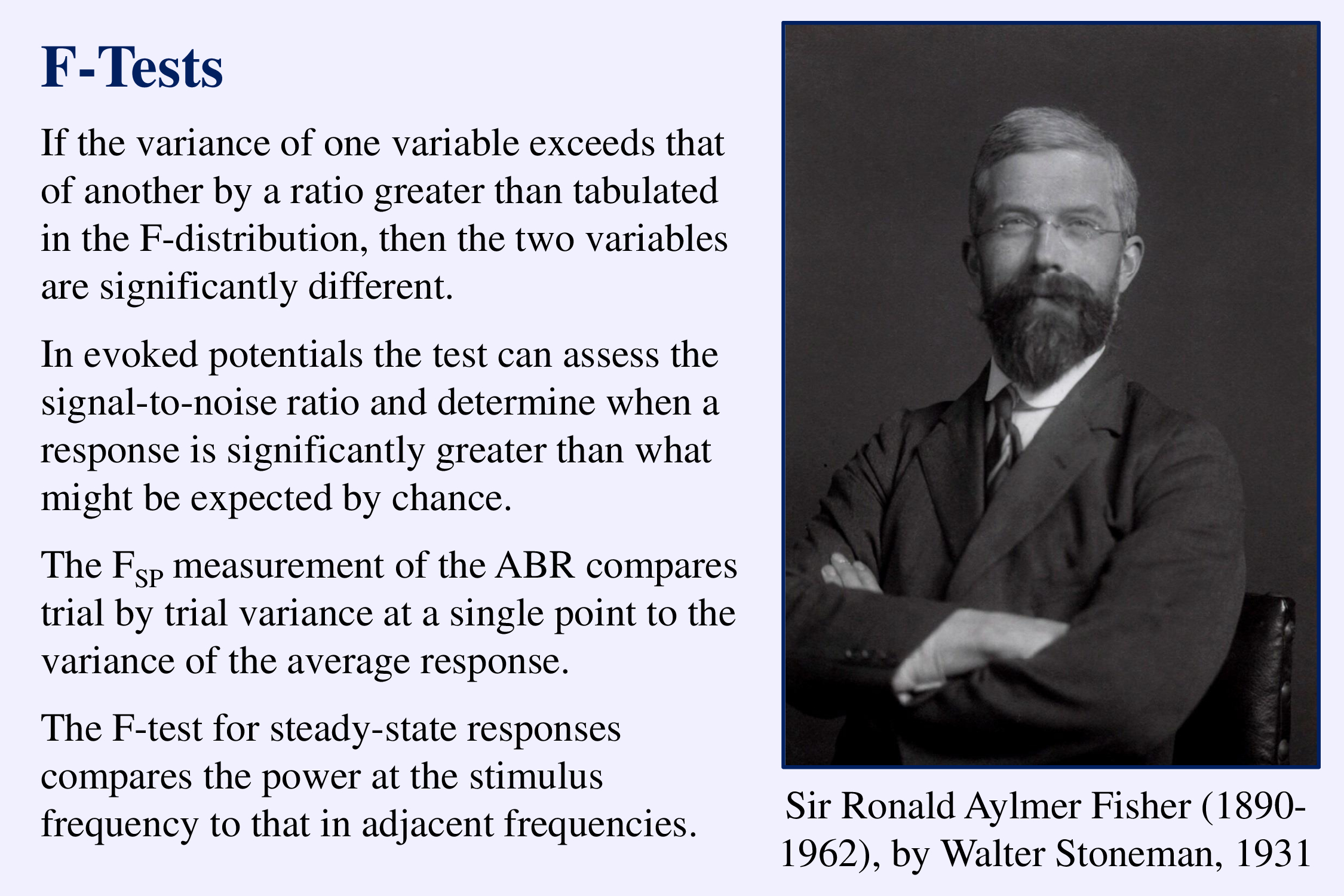
Ronald Fisher was a brilliant mathematician who almost single-handedly established modern scientific statistics. The “F-test” is named after him. When he was right he was really right. And if you use the correct statistical tests you will be as confident in your interpretation as Fisher is in his photograph. You will be unbiased – “objective.” The Fsp test for the auditory brainstem response (ABR) is described in Elberling & Don (1984), and the F-test in steady-state responses is discussed in Dobie and Wilson (1996).
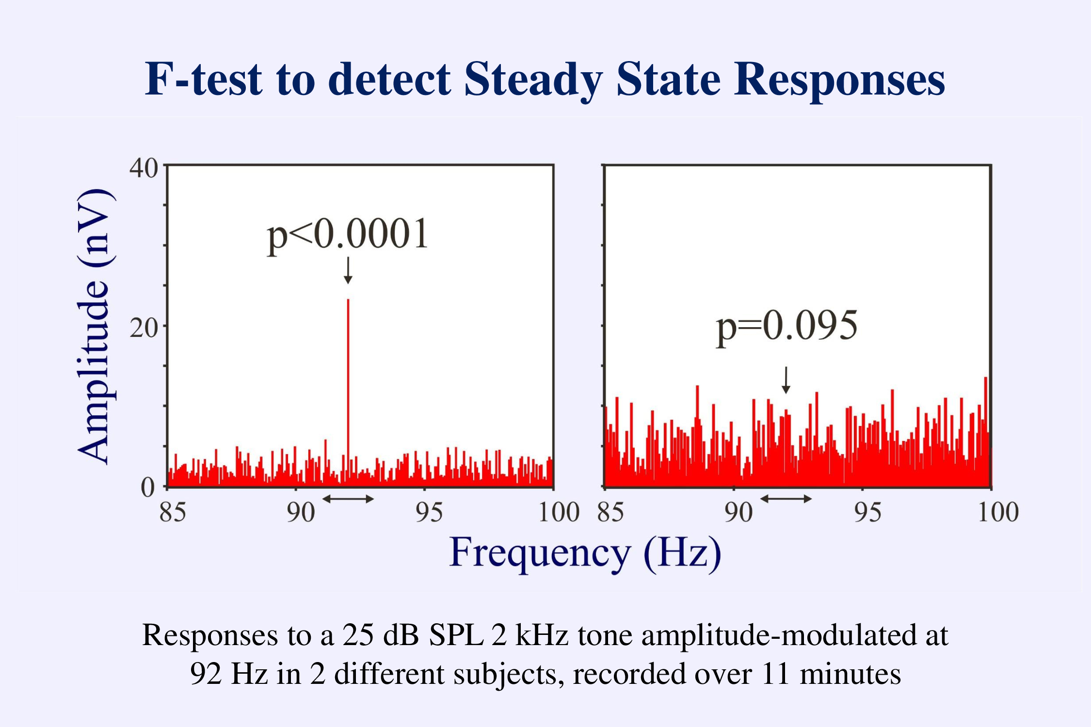
This figure illustrates the use of an F-test to detect a steady-state response. In the frequency domain the steady-state response shows up as a line at the frequency at which the stimuli were presented. The activity at the other frequencies in the spectrum represents the unaveraged background EEG. The F-test compares the amplitude at the stimulus frequency to that at adjacent frequencies. If the stimulus amplitude is significantly larger than what would be expected by chance (left example) we can conclude that there is a response. If not (right example), we can only conclude that the response is not yet greater than the background EEG. We need another criterion – a low level of the background noise – to decide that that response is not present.
In the frequency domain, responses to chirps occur both at the rate of stimulation and at harmonics of this rate. Depending on the subject and the stimulus-rate, some harmonics may be more prominent than others. Combining the statistical tests for the responses at each of the multiple harmonics can give a more reliable test of whether or not a response is present in the recording than simply looking at the response at the fundamental frequency (Cebulla et al., 2006).
b) Threshold-Seeking Algorithms
Once we have a reliable technique for determining whether a response is present or not, we can then determine the threshold for the response. Thresholds can be estimated using fixed or adaptive methods. The fixed method records responses at multiple levels above and below threshold and records the probability of detection as a psychometric function. In an adaptive technique the intensity presented on any one trial depends on the responses to preceding trials (Taylor & Creelman, 1967). For example the intensity can be decreased by 10 dB after a positive response and increased by 5 dB after a negative response:
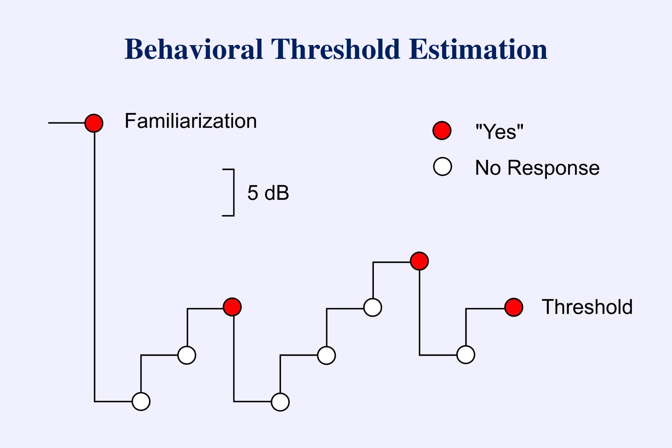
The above diagram represents the usual approach to estimating thresholds in behavioral audiometry (American Speech-Language-Hearing Association, 2005). Initially the subject is familiarized with the stimulus so that he or she knows what to listen for. The tester then starts below threshold and ascends in 5 dB steps until the subject hears the tone. The stimulus is then decreased by 10 dB and the ascent begun again. This down-10-up-5-dB sequence is repeated until a positive response occurs at one level in two out of three trials. This level is then considered threshold.
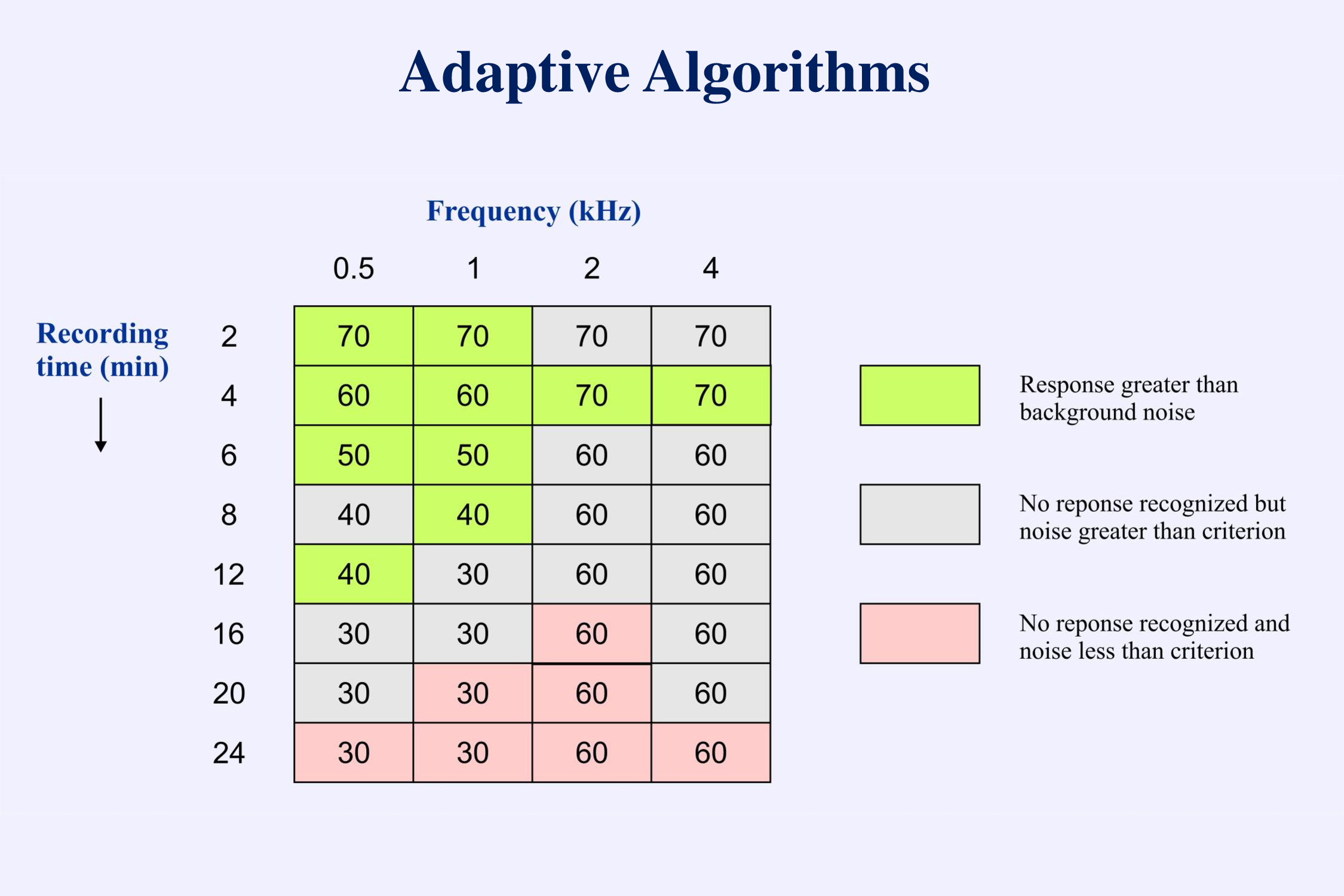
This protocol works well when recording behavioral responses. There is little difference in time between a “yes” response and a “no” response. In recording evoked potentials this approach is not efficient. The problem is that it takes much longer to decide that an electrophysiological response is absent than it takes to decide that the response is present. In the example provided, threshold is determined after 3 positive responses and 6 negative responses. To decide that a response is not present we must continue the averaging until the background EEG noise is below some low criterion. Testing can take a long time if the protocol requires more negative than positive responses. Therefore when estimating thresholds for evoked potentials we usually use a descending technique. Then we only need to spend a long recording time at the end when we have gone below threshold and have to determine that no responses are present. The following set of data (Figure 10-14 from Picton, 2011) illustrates the processes of recognizing responses (arrows) and determining threshold.
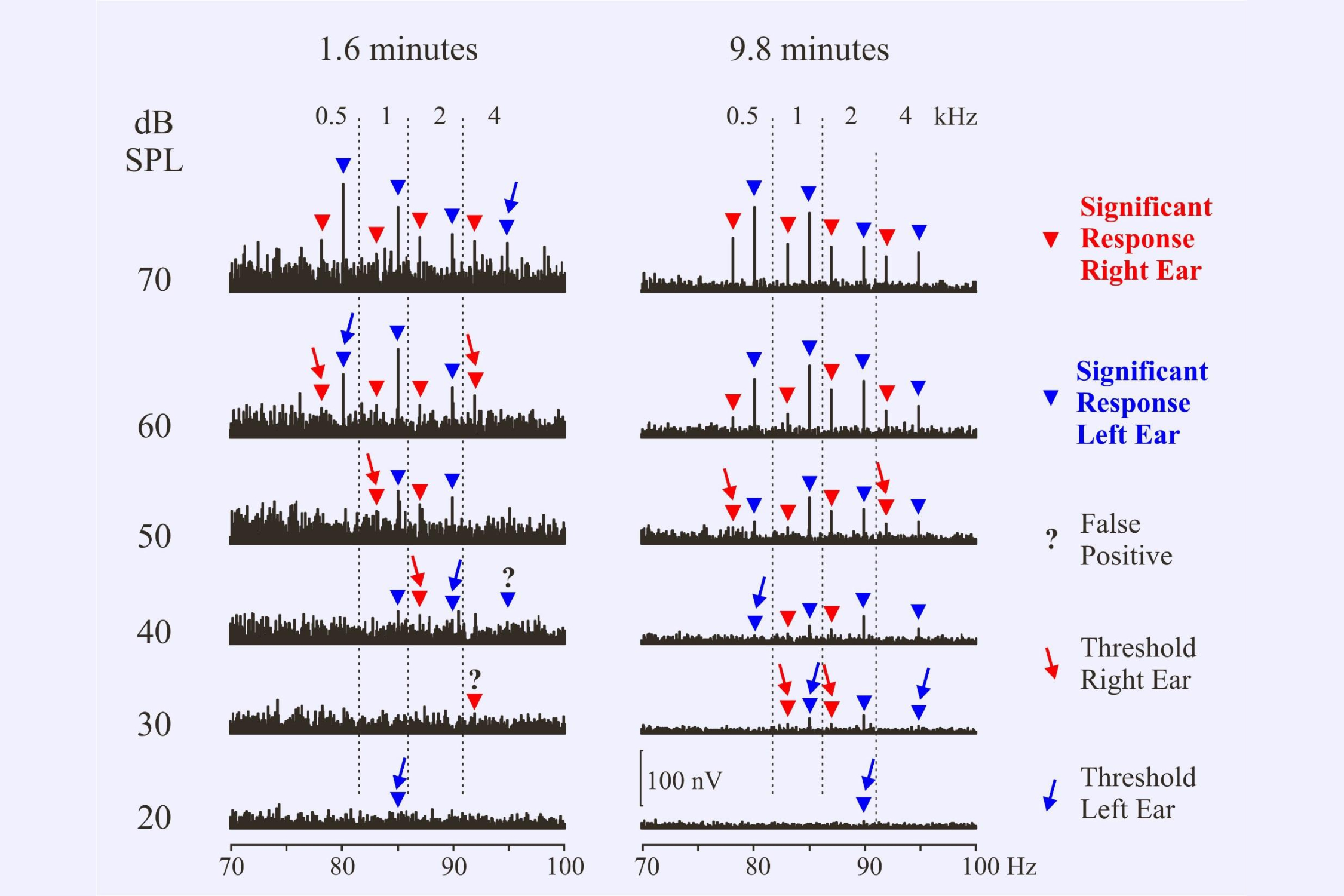
When determining thresholds we need to consider the possibility of false positive responses. Using a test criterion of p=0.05, about 1 in 20 responses could be “detected” even if there were actually no responses present. This is the nature of the statistical test. In the present set of recordings two responses out of 61 were considered to be false positives – designated by the ?
We also need to consider the possibility that a response might be missed. Perhaps the noise in one recording was particularly high. Thus in the illustration we might consider the 1 kHz response at 30 dB in the 1.6 minute recording to have been inadvertently missed because there is a response at 20 dB. Or perhaps the response at 20 dB is another false positive. Decisions! Decisions!
A major question is whether we should continue to recording to a set time – say 10 minutes – or whether we can stop as soon as all responses are recognized – e.g. after 1.6 minutes. At 70 dB SPL all responses are recognized after 1.6 minutes of averaging. There would be no need to continue longer at this intensity.
To save time, can we just stop the recording once a response is detected? Can we watch the ongoing response, monitor the significance level and then stop when criterion is reached? The problem with this approach is that the more times we test for significance the greater the probability that we might reach criterion level by chance. A significance level of p<0.05 means that we would judge a response significant 1 in 20 times even though there was no response present. If we check the responses more than 20 times we should expect some false detections.
We can compensate for this using various statistical corrections. A simple Bonferroni correction divides the probability criterion by the number of tests. The following illustration (Figure 6-14 from Picton, 2011) shows the corrected criterion when monitoring the significance level every minute or every 4 seconds. The correction is more severe when the monitoring is more frequent. The response is to a 1 kHz amplitude modulated tone at low intensity (25 dB SPL) in two different subjects. In the upper subject the response becomes significant in 2 minutes using 1 minute monitoring and in 5.2 minutes using 4-second monitoring. In the lower subject the response never reaches significance using the 4-second monitoring protocol.
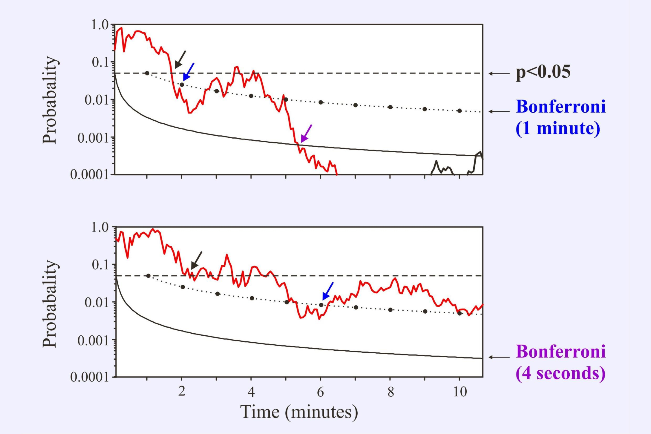
Cebulla and Stürzebecher (2015) have recently proposed protocols wherein the interval between the statistical tests increases over time. If the response is not significant the protocol waits longer before testing again.
c) Physiological and Behavioral Thresholds
The lowest intensity at which an evoked potential is detected is the “physiological threshold.” Since this is higher than the behavioral threshold, we normally subtract a “correction factor” – the mean physiological-behavioral difference – to obtain an “estimated behavioral threshold.”
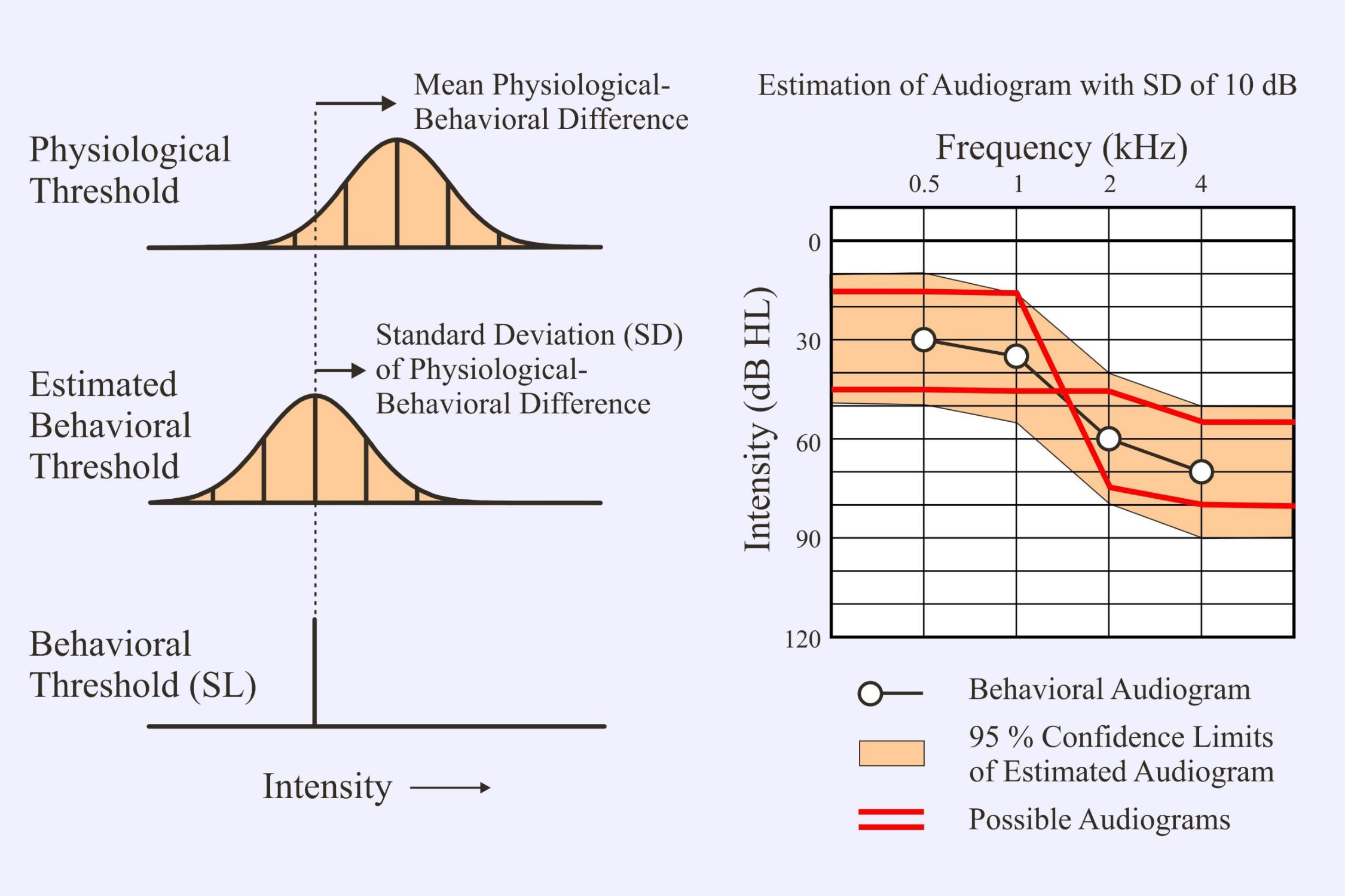
It is important to note the standard deviation (SD) of the correction factor since this will determine the range for the actual behavioral threshold. One normally assumes that the range is ±2SD – this would include 95% of the possible values. The SD of the correction factors has usually been around 10 dB. This means that we could be out in our estimated behavioral threshold by up to 20 dB in either direction. In the above example the hypothetical patient could actually have either a flat audiogram or a limited high-frequency loss (Figure 6-15 from Picton, 2011). The most recent reports for multiple auditory steady state responses with chirps (e.g., Sininger et al, 2018) give SDs of 5-8 dB. These are much better.
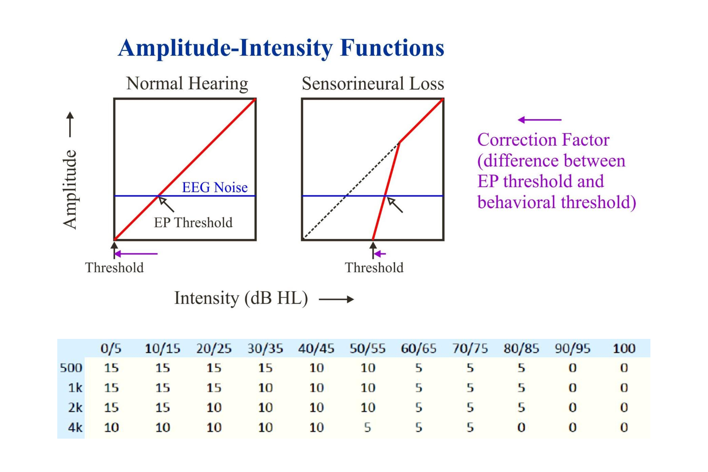
Correction factors decrease as the threshold intensity increases. This is due to the response amplitude (like the perceived intensity) increasing more quickly above threshold when there is a hearing loss (upper half of the above illustration). The lower table gives sample correction factors for the 40 Hz steady state responses to chirps: 10 to 15 dB at low intensities and 0 dB at high.
At present most systems using multiple steady state responses present all the stimuli at one intensity. In some systems one can separately adjust the intensity of each stimulus. Once a significant response has been detected, the intensity can be lowered. Or if no response has been detected and the background noise has reached a criterion level, the test may be stopped or the intensity increased. These ideas were initially examined by Roland Muehler and his colleagues (2012). The only caution in this approach is that the difference in intensities between stimuli should likely not exceed 30 dB so that there is no masking of one stimulus by the others (John et al., 2002). The following illustration suggests how this might occur in assessing a high-frequency hearing loss:
What is needed is for this procedure to be made completely automatic – for the system’s algorithms (rather than the audiologist) to decide when to change the intensity as well as to decide whether a response is present or not. Then we would have completely objective audiometry – objective on the part of the patient and objective on the part of the examiner.
d) Sweep Techniques
The following figure illustrates the idea of using sweeps of intensity to evaluate thresholds (Picton et al., 2007). It shows shows the following response to a 2 kHz stimulus amplitude modulated at 92 Hz that over 16 seconds ascends in intensity from 25 dB SPL to 75 dB and then decreases back to 25 dB. In the upper left is shown the spectrogram – the response can be seen coming out of the background EEG noise near the beginning of the sweep, increasing in amplitude and then decreasing until it is no longer recognizable.
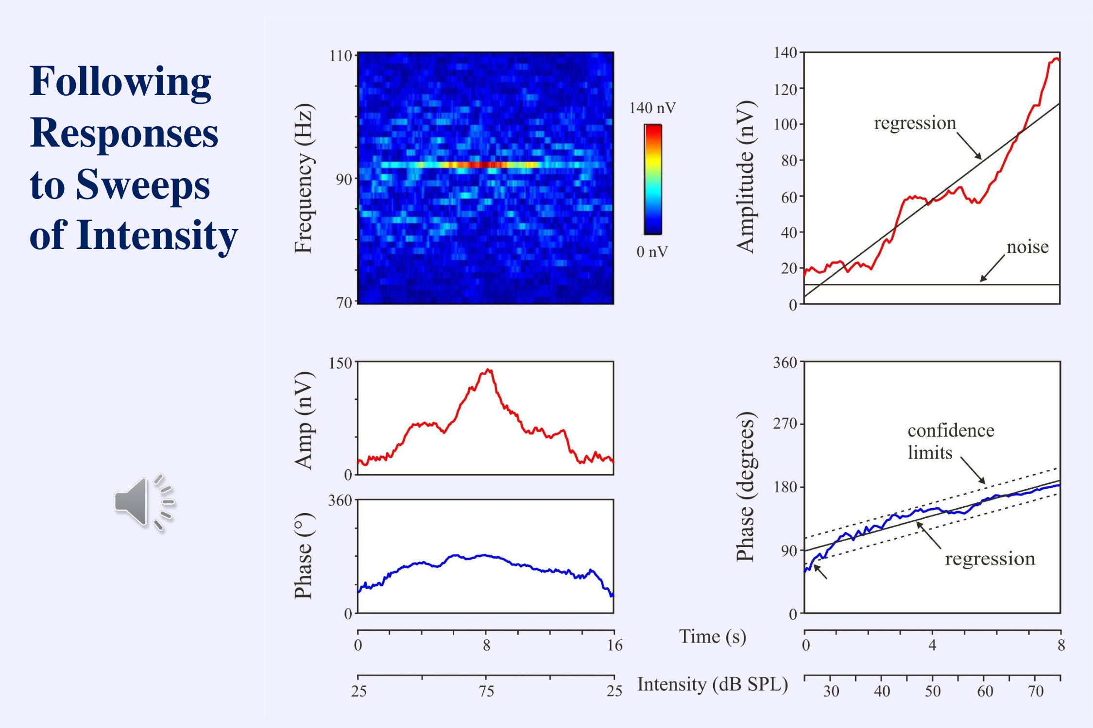
The graphs demonstrate the effects of intensity on the amplitude and phase of the response. The advantage of the sweep technique is that you can use the recorded amplitudes and phases to plot an amplitude-intensity function and extrapolate to threshold.
My dream is that the algorithms for assessing thresholds will sweep back and forth over and above threshold, narrowing the range of intensity until the threshold is accurately and automatically bracketed. One of the dreams of an old man.
Conclusions – Threshold Detection
We have good techniques to monitor the responses so that we can recognize them quickly and accurately.
What we still need are some automatic threshold-seeking algorithms that can vary the intensity among the different stimuli.
IV. Speech Perception
Now we turn to the final topic– the objective assessment of speech perception. In recent years there has been a revolution in auditory science (Hamilton & Huth, 2018). Rather than using clicks and tones to examine how the auditory system works, scientists are using speech stimuli. This makes sense. Human auditory systems have evolved to process speech – not clicks and tones.
a) Assessing Hearing Impairment and Fitting Hearing Aids
In audiology we should move “beyond the audiogram” and pay more attention to speech perception (Fabry 2015). Our patients come to us complaining that they cannot understand when others speak to them. They do not complain that they are unable to hear clicks and tones. We should evaluate how well they perceive speech – in quiet and in noise (Dubno, 2018; Soli et al, 2018ab).
Speech stimuli can be particularly important in audiology when fitting hearing aids to compensate for a hearing impairment. The goal is to amplify the speech signal and compress it to fit within the range of what is comfortably audible:
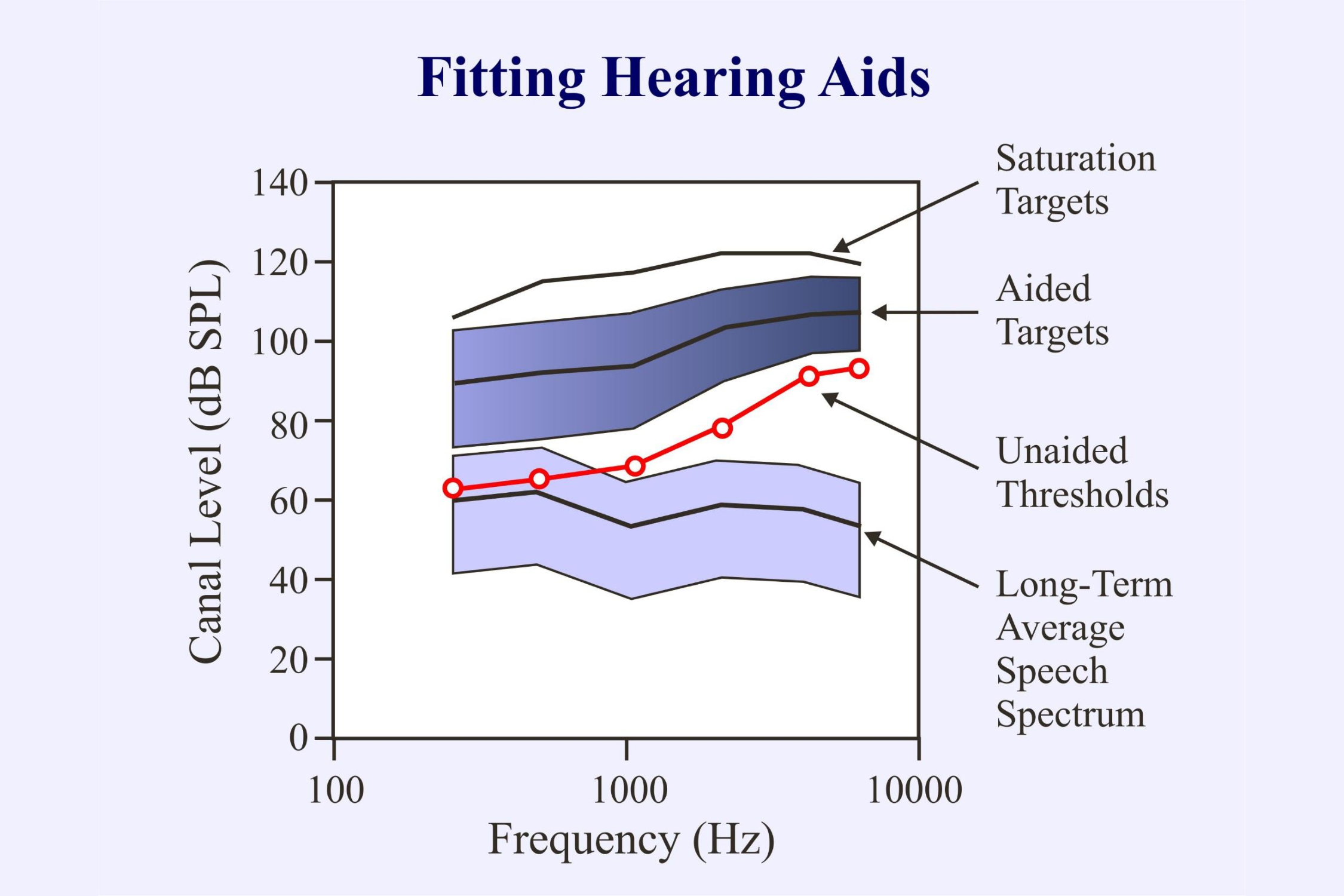
In objective audiometry we can derive the unaided thresholds from chirp-evoked auditory steady state responses. We can also evaluate the responses of the brain to aided stimuli (Laugesen, et al., 2018; Picton et al., 1998). However, hearing aids were not designed to amplify chirps or tones. They are set up to amplify speech. They would be better evaluated using speech sounds.
b) Frequency Following Responses
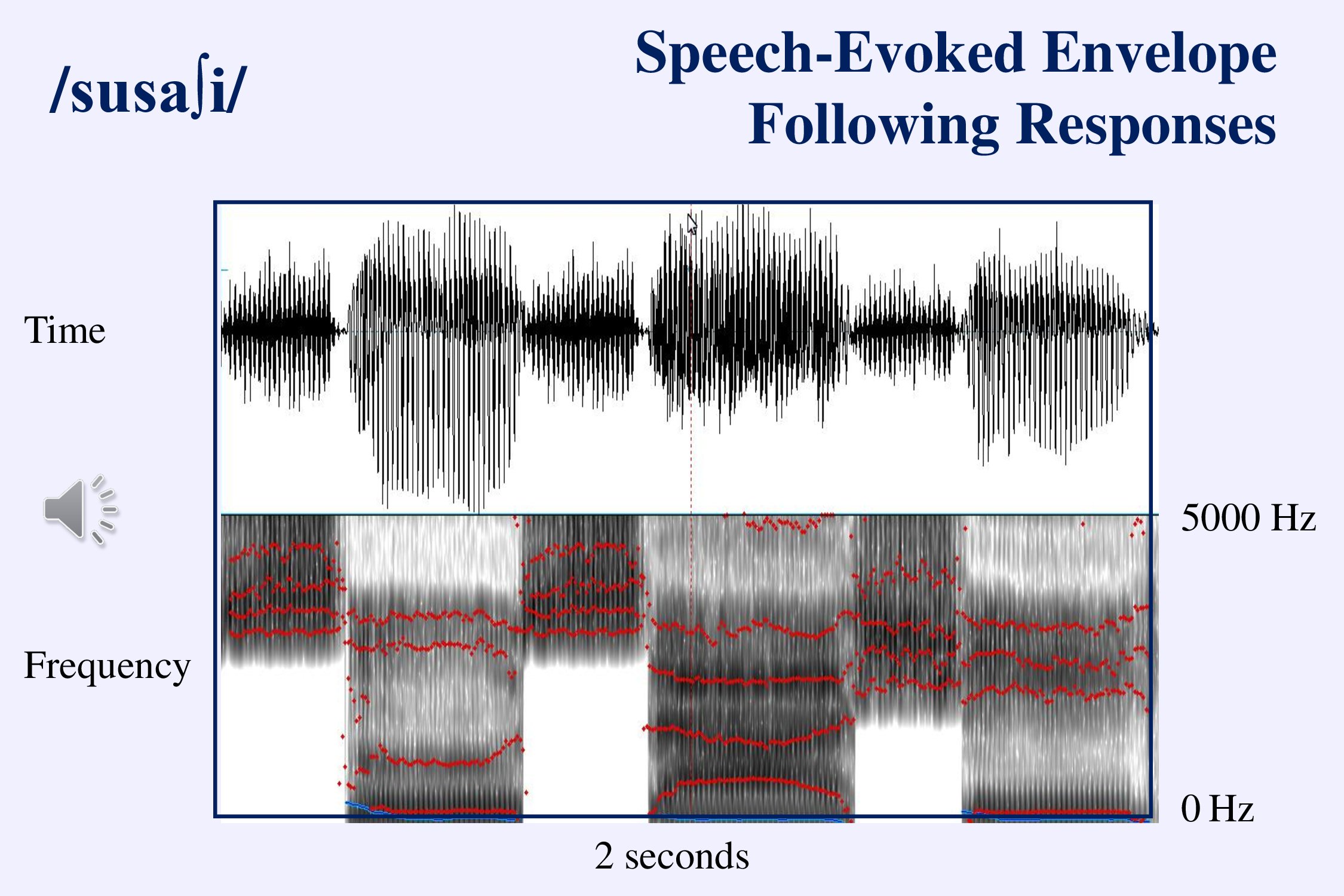
A simple way to assess the brain’s ability to process speech sounds is to record frequency- and envelope-following responses to simple speech stimuli like vowels (Aiken & Picton, 2008a; Krishnan, 2007, 2017; Ribas-Prats et al, 2019). If these speech stimuli are accurately reproduced by the brainstem we can be sure that the stimuli have been properly processed in the cochlea and are available to be discriminated.
One fascinating aspect of the speech FFRs concern the ability of adults and infants to follow the pitch changes that are phonetically meaningful in tonal languages like Chinese (Krishnan et al., 2004; Jeng et al., 2016).
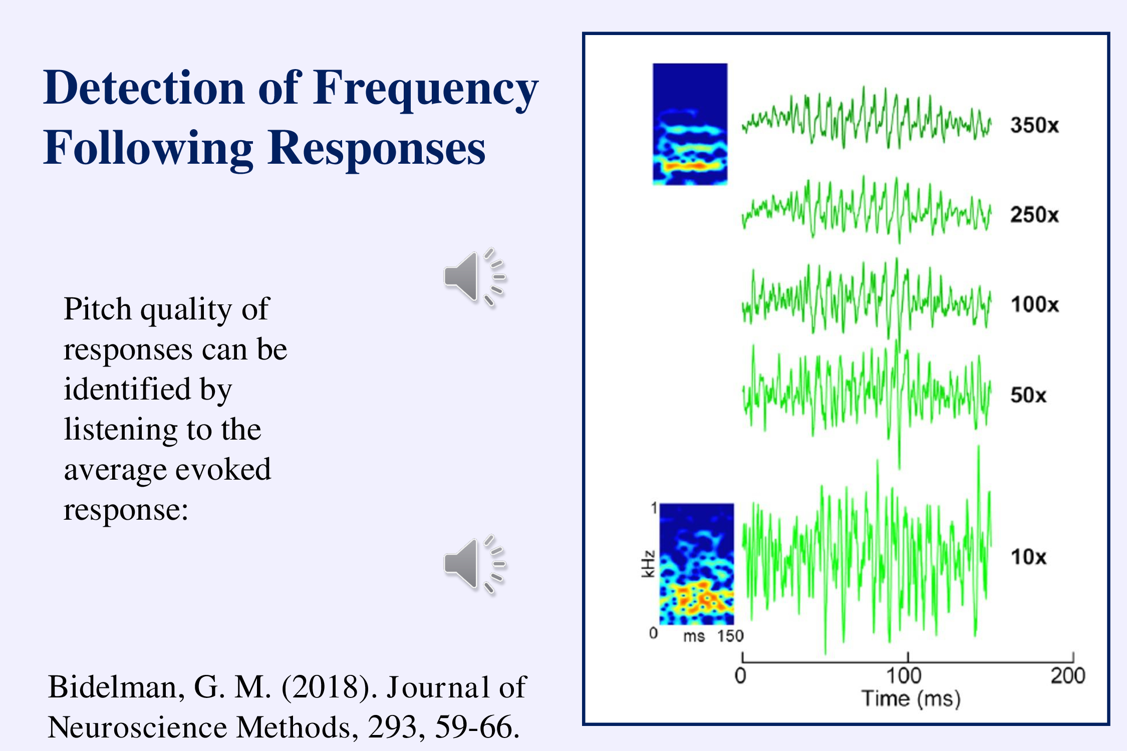
Another interesting aspect of using speech stimuli is that we can listen to the response played back into a speaker and recognize easily when the response is there (Bidelman, 2018a). The examples illustrate early in the recording and late in the recording. As the recording progresses you can hear the /a/ sound in the background noise:
Viji Easwar and her colleagues have been considering a stimulus that uses several different speech sounds as a way to evaluate the ability of a hearing aid to transfer speech information to the brain (Easwar et al., 2015ab). The frequencies in this stimulus cover the range of the long term speech spectrum. The idea is to evaluate envelope- and frequency-following response to these amplified sounds to assess how well a hearing aid makes speech audible.
One difficulty with these recordings is that several different regions of the auditory pathway from cochlea to cortex generate frequency-following responses and these have different phase relations to the stimulus (Bidelman, 2018b; Easwar et al., 2018; King et al., 2016). Sometimes the fields from different generators may be out of phase and thus cancel themselves.
c) Following the Speech Envelope
The brainstem frequency following response tracks the envelope of speech sounds, portraying how the pitch and the formants change over time. This can give the phonetic structure of speech. Another aspect of speech is the overall speech envelope – how the amplitude changes over time at rates of 1-10 Hz. Shannon and his colleagues (1995) demonstrated how important this is to the recognition of ongoing speech. Magnetoencephalographic data indicated that the human auditory cortex follows this speech envelope (Ahissar et al. 2001).
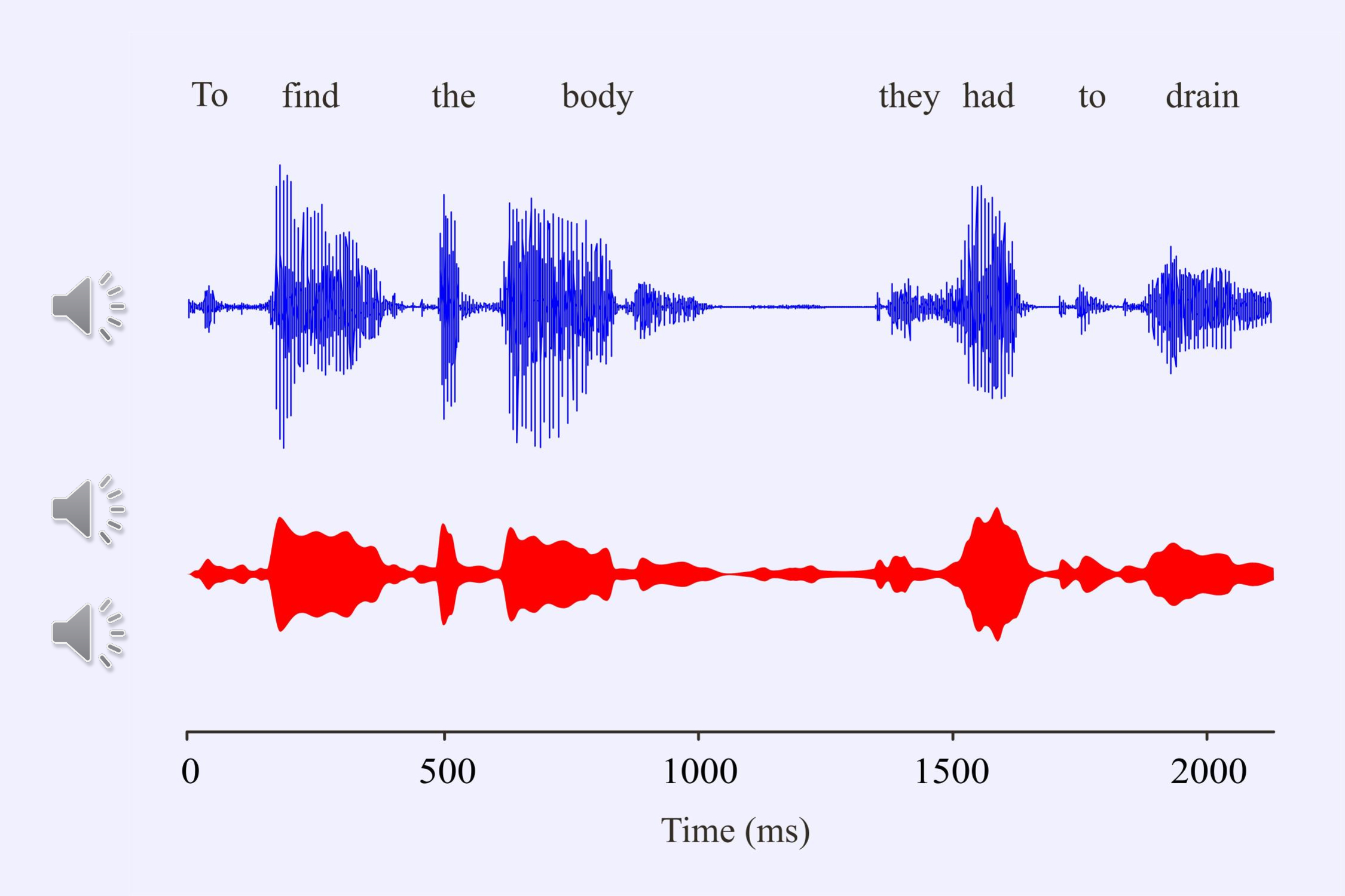
Aiken and I (2008b) decided to record electroencephalographic responses to the speech envelope of several sentences such as “To find the body they had to drain the (lake).” The sentence comes from a detective story. The last word is missing since we had to ensure that the subjects attended to the sentence when it was repeated. We ended the sentence either with the correct word or with an incongruous word.
If you take the envelope of a spoken sentence, and fill it with octave-band filtered versions of the original sentence, you can likely still understand it even though it has no pitch and little frequency information. It sounds like whispering. If you fill the envelope with white noise, the rhythm of the sentence is still preserved. The human brain likely uses the overall amplitude of the speech envelope to divide the speech up into recognizable chunks – syllables and words.
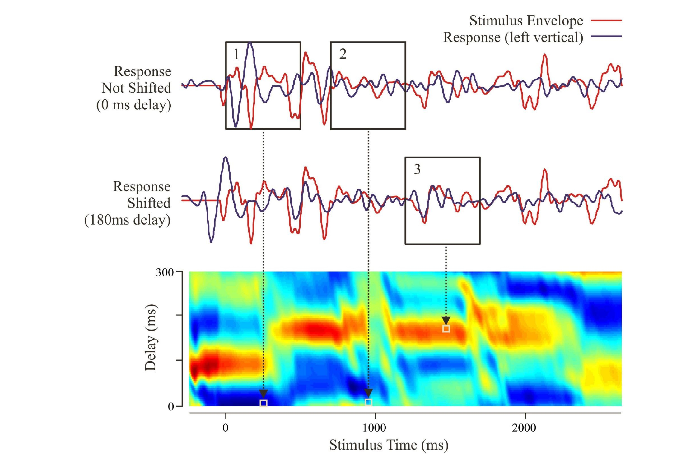
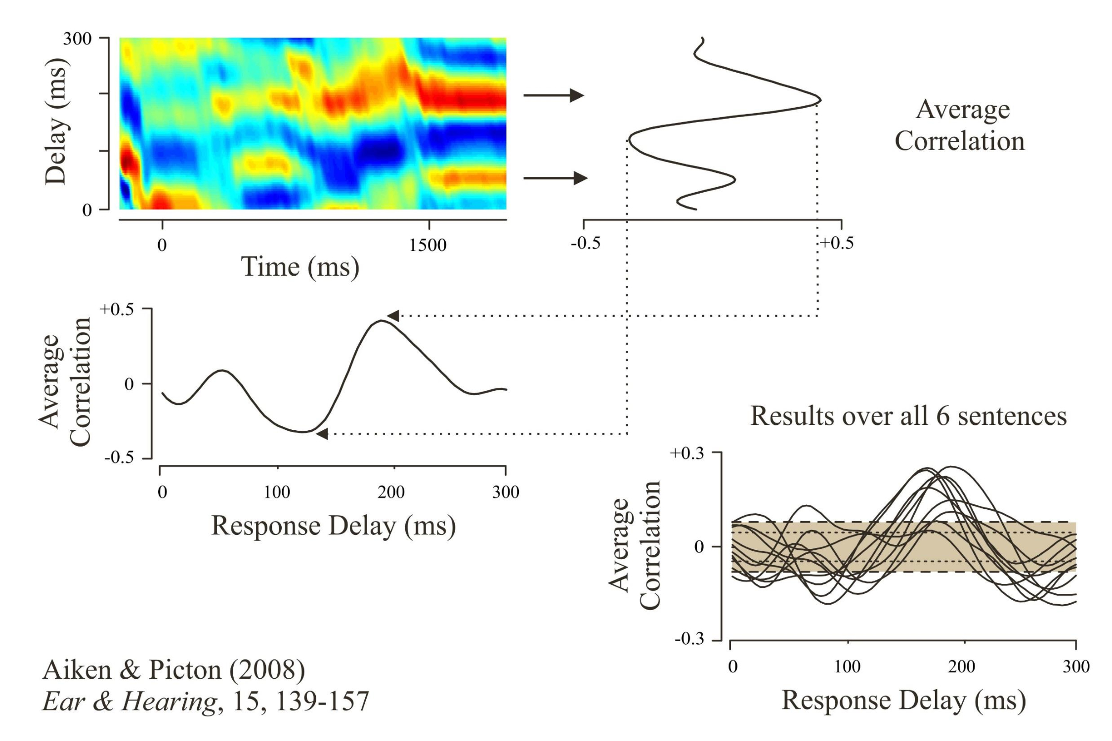
Basically we presented 6 different sentences, averaged the response to each sentence over multiple repetitions, and derived source waveforms from the left and right auditory cortex. We then correlated the source waveform to the speech envelope, using variable delays. The correlation was highest when the speech envelope occurred between 100 and 200 ms before the source waveform (red regions).
We could then average the correlations over the period of the sentence to give a “transfer function.” This was significantly greater than what would occur by chance (shaded area). The human auditory cortex followed the speech envelope with a delay between 100 and 200 milliseconds. As I speak your auditory cortex is following me.
d) Development of Speech and Language
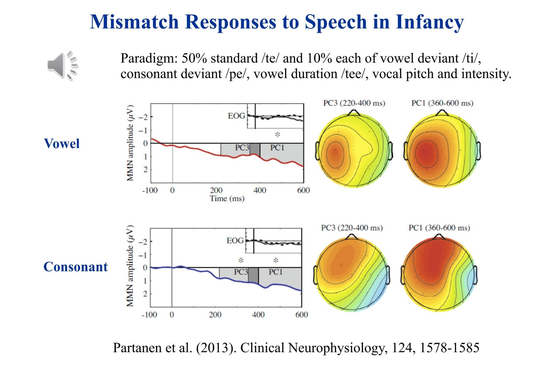
However, following the speech envelope does not mean that we can understand what is being said. For that we need to discriminate the different speech sounds. One way to see whether the brain recognizes the difference between speech sounds is to record the mismatch response to a phonetic change. We mentioned this earlier in the talk – remember ba….ba….baa….ba. Unfortunately it takes a long time to record the mismatch response to a single phonetic change.
Recently, Partanen and his colleagues (2013) have shown that many different mismatch responses may be recorded concurrently to different speech sounds in young infants. Five different mismatches were run concurrently. The actual sound sample includes only the consonant change /te/ to /ti/, the intensity change and the change in vowel duration. The recordings show significant mismatch responses to the phonetic changes. Again negativity is plotted upward in this illustration. For these infants the Mismatch Response was a slow positive wave.
A major problem remains about using the mismatch response in infancy and childhood. We need to figure out when the infant response is positive and when negative. How does this depend on the state of arousal and the age of the child? And we need to track the development of the mismatch response over childhood.
Angela Friederici (2005) has proposed that infants show a progressive development of language capabilities: the discrimination of phonemes in the language to which they have been exposed, the recognition of prosodic features, the identification of words, and finally the structuring of syntax.
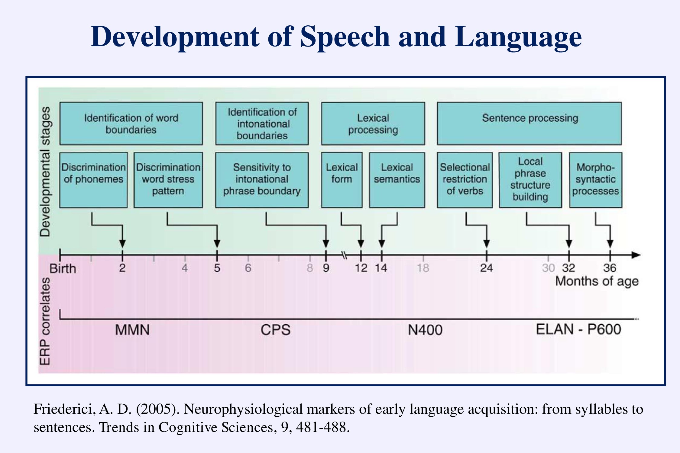
This development can be followed using the auditory evoked potentials. I have illustrated the mismatch negativity (MMN). The CPS – closure positive shift – occurs at the end of sentences or phrases. The N400 occurs when the words don’t make sense. The ELAN early left anterior negativity – and the P600 – occur with grammatical errors. We need to set up standard paradigms to assess the development of speech and language in infants and young children.
e) Multivariate Temporal Response Functions
So now for another dream. Recently sophisticated mathematical techniques have been developed to determine the ability of the human brain to follow speech – most particularly “multivariate temporal response functions” (mTRF). These techniques can demonstrate EEG entrainment to the speech envelope, and also to the phonetic changes that are occurring during the ongoing speech (Ding & Simon, 2014; Lalor & Foxe, 2010). The degree of correlation determined using these techniques can relate to the ability of the subject to recognize speech (Vanthornhout et al., 2018).
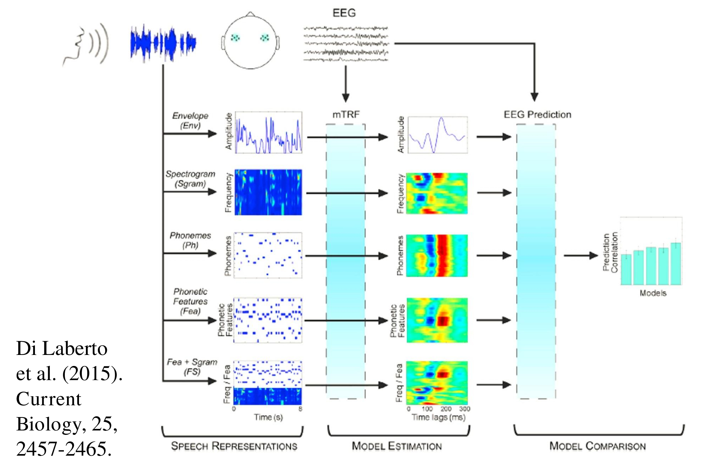
Recent years have seen a plethora of papers using these new statistical techniques to measure how the brain follows various aspects of the speech signal (Brodbeck et al., 2018; Di Liberto et al., 2015, 2017; Kalashnikova et al., 2018;.Trng et al, 2017, 2018; Wöstmann et al, 2017). With more research we might be able to present natural ongoing speech to a patient and obtain an objective measure of speech perception.
Conclusions – Speech Perception
Following responses can evaluate how speech is being processed in the brain.
What we still need is some objective test of speech discrimination. I have mentioned the MMN. We also need to study the development of other late evoked potentials that process speech and language.
Summary
I have briefly reviewed the need for objective audiometry – for both pure tone thresholds and for speech perception. I have proposed the principle of multiplicity – many stimuli at the same time, and many different responses for each stimulus. I discussed how thresholds can be objectively recognized, and proposed automatic algorithms to reach threshold – our testing should be as objective for the examiner as for the patient. Finally I suggested some ways in which we can assess speech perception – using following responses and the mismatch response.
In objective audiometry, I long for the day when pure tone thresholds are accurately and quickly assessed without any intervention on my part, and when I can speak to a patient and see through his electroencephalogram whether he or she is following what I am saying. I am getting old and it is the prerogative of the elderly to dream.
Acknowledgments
My sincere thanks to colleagues who provided me with sounds, papers, ideas and advice: Steve Aiken, Gavin Bidelman, Mario Cebulla, Andrew Dmitrijevic, Andrée Durieux-Smith, Viji Easwar, Claus Elberling, Angela Friederici, Sasha John, Nina Kraus, Otavio Lins, Roland Muehler, Eino Partanen, Marilyn Perez-Abalo, David Purcell, Yvonne Sininger, Susan Small, David Stapells, Andy Stuart, Martin Walger, Jan Wouters.
References
Ahissar, E., Nagarajan, S., Ahissar, M., Protopapas, A., Mahncke, H., Merzenich, M.M. (2001) Speech comprehension is correlated with temporal response patterns recorded from auditory cortex. Proceedings of the National Academy of the Sciences United States of America, 98, 13367-13372.
Aiken, S.J., & Picton, T.W. (2008a). Envelope and spectral frequency following responses to vowel sounds. Hearing Research, 245, 35-47.
Aiken, S.J., & Picton, T.W. (2008b). Human cortical responses to the speech envelope. Ear and Hearing, 15, 139-157.
American Speech-Language-Hearing Association. (2005). Guidelines for manual pure-tone threshold audiometry.
Anderson, S., Parbery-Clark, A., White-Schwoch, T., & Kraus, N. (2015). Development of subcortical speech representation in human infants. Journal of the Acoustical Society of America. 137(6), 3346-3355.
Baljić, I., Eßer, D., Foerst, A. & Walger, M. (2017). Evaluation of optimal masking levels in place-specific low-frequency chirp-evoked auditory brainstem responses. Journal of the Acoustical Society of America, 141, 197–206.
Bidelman, G. M. (2015). Towards an optimal paradigm for simultaneously recording cortical and brainstem auditory evoked potentials. Journal of Neuroscience Methods, 241, 94–100.
Bidelman, G. M. (2018a). Sonification of scalp-recorded frequency-following responses (FFRs) offers improved response detection over conventional statistical metrics. Journal of Neuroscience Methods, 293, 59-66.
Bidelman, G. M. (2018b). Subcortical sources dominate the neuroelectric auditory frequency-following response to speech. NeuroImage, 175, 56-69.
Bidelman, G. M., Pousson, M., Dugas, C., & Fehrenbach, A. (2018). Test-retest reliability of dual-recorded brainstem vs. cortical auditory evoked potentials to speech. Journal of the American Academy of Audiology, 29, 164–174.
BinKhamis G, Léger A, Bell SL, Prendergast G, O’Driscoll M, & Kluk K. (2019, in press) Speech auditory brainstem responses: effects of background, stimulus duration, consonant–vowel, and number of epochs. Ear & Hearing.
Brodbeck, C., Presacco, A., & Simon, J.Z. (2018). Neural source dynamics of brain responses to continuous stimuli: Speech processing from acoustics to comprehension. NeuroImage, 172:162-174.
Byrne, D., Dillon, H., Tran, K., Arlinger, S., Wibraham, K., Cox, R., Hagerman, B., Hetu, R., Kei, J., Lui, C., Kiessling, J., Kotby, M., Nasser, N., El Kholy, W., Nakanishi, Y., Oyer, H., Powell, R., Stephens, D., Meredith, R., Sirimanna, T., Tavatkiladze, G., Frolenkov, G., Westerman, S. & Ludvigsen, C (1994). An international comparison of long-term average speech spectra. Journal of the Acoustical Society of America, 96 2108-2120.
Cebulla, M., & E. Sturzebecher, E. (2015). Automated auditory response detection: Further improvement of the statistical test strategy by using progressive test steps of iteration. International journal of audiology, 54, 568-572.
Cebulla, M., Stürzebecher, E., Don, M., & Müller-Mazzotta J. (2012). Auditory brainstem response recording to multiple interleaved broadband chirps. Ear & Hearing, 33, 466-479.
Cebulla, M., Stürzebecher, E., & Elberling, C. (2006). Objective detection of auditory steady-state responses: Comparison of one-sample and q-sample tests. Journal of the American Academy of Audiology, 17, 93–103.
Cobb, K.M., & Stuart, A. (2016a). Neonate auditory brainstem responses to CE-chirp and CE-chirp octave band stimuli II: versus adult auditory brainstem responses. Ear and Hearing, 37, 724-743.
Cobb, K.M., & Stuart, A. (2016b). Neonate auditory brainstem responses to CE-chirp and CE-chirp octave band stimuli I: versus click and tone burst stimuli. Ear and Hearing, 37, 710-723.
Cobb, K.M., & Stuart, A. (2016c). Auditory brainstem response thresholds to air- and bone-conducted CE-Chirps in neonates and adults. Journal of Speech, Language, and Hearing Research, 59, 853-859.
Ding, N., & Simon, J. Z. (2014). Cortical entrainment to continuous speech: functional roles and interpretations. Frontiers in Human Neuroscience, 8, 311.
Di Liberto, G.M., O’Sullivan, J.A., & Lalor, E.C. (2015). Low-frequency cortical entrainment to speech reflects phoneme-level processing. Current Biology, 25, 2457–2465.
Di Liberto, G. & Lalor, E. (2017). Indexing cortical entrainment to natural speech at the phonemic level: Methodological considerations for applied research. Hearing Research, 348, 70-77.
Dobie, R. A., & Wilson, M. J. (1996). A comparison of t test, F test, and coherence methods of detecting steady-state auditory-evoked potentials, distortion-product otoacoustic emissions, or other sinusoids. Journal of the Acoustical Society of America, 100, 2236-2246.
Dubno, J. R. (2018). Beyond the audiogram: application of models of auditory fitness for duty to assess communication in the real world. Ear & Hearing, 39(3), 434-435.
Easwar, V., Purcell, D. W., Aiken, S. J., Parsa, V., & Scollie, S. D. (2015a). Effect of stimulus level and bandwidth on speech-evoked envelope following responses in adults with normal hearing. Ear and Hearing, 36(6), 619-634
Easwar, V., Purcell, D. W., Aiken, S. J., Parsa, V., & Scollie, S. D. (2015b). Evaluation of speech-evoked envelope following responses as an objective aided outcome measure: effect of stimulus level, bandwidth, and amplification in adults with hearing loss. Ear and Hearing, 36(6), 635-652.
Easwar, V., Banyard, A., Aiken, S.J., & Purcell, D.W. (2018). Phase-locked responses to the vowel envelope vary in scalp-recorded amplitude due to across-frequency response interactions. European Journal of Neuroscience, 48(10), 3126-3145.
Elberling, C., & Don, M. (1984). Quality estimation of averaged auditory brainstem responses. Scandinavian Audiology, 13, 187–197.
Elberling, C., & Don, M. (2010). A direct approach for the design of chirp stimuli used for the recording of auditory brainstem responses. Journal of the Acoustical Society of America, 128, 2955–2964.
Elberling, C., & Crone-Esmann, L. (2017). Calibration of brief stimuli for the recording of evoked responses from the human auditory pathway. Journal of the Acoustical Society of America, 141, 466-474.
Fabry, D. A. (2015). Moving beyond the audiogram. Audiology Today, 27 (3), 34-39.
Ferm, I., Lightfoot, G., & Stevens J. (2013). Comparison of ABR response amplitude, test time, and estimation of hearing threshold using frequency specific chirp and tone pip stimuli in newborns. International Journal of Audiology, 52, 419-423.
Ferm, I., & Lightfoot, G. (2015). Further comparisons of ABR response amplitudes, test time, and estimation of hearing threshold using frequency-specific chirp and tone pip stimuli in newborns: Findings at 0.5 and 2 kHz. International Journal of Audiology, 54, 745–750
Frank, J., Baljić, I., Hoth, S., Eßer, D., & Guntinas-Lichius, O. (2017). The accuracy of objective threshold determination at low frequencies: comparison of different auditory brainstem response (ABR) and auditory steady state response (ASSR) methods. International Journal of Audiology, 56, 337-345.
Friederici, A. D. (2005). Neurophysiological markers of early language acquisition: from syllables to sentences. Trends in Cognitive Sciences, 9, 481-488
Friederici, A. D., Friedrich, M., & Weber, C. (2002). Neural manifestation of cognitive and precognitive mismatch detection in early infancy. NeuroReport, 13, 1251-1254.
Gøtsche-Rasmussen, K., Poulsen, T., & Elberling, C. (2012). Reference hearing threshold levels for chirp signals delivered by an ER-3A insert earphone. International Journal of Audiology, 51, 794-799.
Hamilton, L. S., & Huth, A. G. (2018): The revolution will not be controlled: natural stimuli in speech neuroscience. Language, Cognition and Neuroscience.
Holube, I., Fredelake, S., Vlaming, M., & Kollmeier, B. (2010). Development and analysis of an International Speech Test Signal (ISTS). International Journal of Audiology, 49(12), 891–903.
Hoth, S., Mühler, R., Neumann, K., & Walger, M. (2014). Objektive Audiometrie im Kindesalter. Berlin: Springer.
Jeng, F.C., Lin, C.D., & Wang, T.C. (2016). Subcortical neural representation to Mandarin pitch contours in American and Chinese newborns. Journal of the Acoustical Society of America, 139, 190-195.
John, M.S., Purcell, D.W., Dimitrijevic, A., & Picton, T. W. (2002). Advantages and caveats when recording steady-state responses to multiple simultaneous stimuli. Journal of the American Academy of Audiology, 13, 246-259.
Johnson, K. L., Nicol, T. G., & Kraus, N. (2005). Brain stem response to speech: a biological marker of auditory processing. Ear & Hearing, 26, 424-434.
Johnson, K. L., Nicol, T., Zecker, S. G., Bradlo, A. R., Sko, E., & Kraus, N. (2008). Brainstem encoding of voiced consonant–vowel stop syllables. Clinical Neurophysiology, 119, 2623–2635.
Kalashnikova, M., Peter, V., Di Liberto, G.M., Lalor, E.C., & Burnham, D. (2018). Infant-directed speech facilitates seven-month-old infants’ cortical tracking of speech. Scientific Reports, 8, Article number: 13745.
King, A., Hopkins, K., & Plack, C. J (2016). Differential group delay of the frequency following response measured vertically and horizontally. Journal of the Association for Research in Otolaryngology, 17, 133–143.
Krishnan, A. (2007). Human frequency following response. In R. F. Burkard, M. Don, & J. J. Eggermont (Eds.), Auditory evoked potentials: Basic principles and clinical application. (pp. 313–335). Baltimore: Lippincott Williams & Wilkins.
Krishnan, A. (2017). Shaping brainstem representation of pitch-relevant information by language experience. In N. Kraus, S. Anderson, T. White-Schwoch, R. R. Fay & A. N. Popper (Eds.). The frequency-following response: a window into human communication. (pp. 45-73). Cham, Switzerland: Springer International.
Krishnan, A., Xu, Y., Gandour, J., & Cariani, P. A. (2004). Human frequency-following response: Representation of pitch contours in Chinese tones. Hearing Research, 189, 1–12.
Lalor, E. C., & Foxe, J.J. (2010). Neural responses to uninterrupted natural speech can be extracted with precise temporal resolution. European Journal of Neuroscience, 31, 189-193.
Laugesen, S., Rieck, J.E., Elberling, C., Dau, T., & Harte, J.M. (2018). On the cost of introducing speech-like properties to a stimulus for auditory steady-state response measurements. Trends in Hearing, 22, 1-11.
Lins, O.G., & Picton, T.W. (1995). Auditory steady-state responses to multiple simultaneous stimuli. Electroencephalography and clinical Neurophysiology, 96, 420-432.
Lins, O.G., Picton, T.W., Boucher, B., Durieux-Smith, A., Champagne, S.C., Moran, L.M., Perez-Abalo, M.C., Martin, V., & Savio, G. (1996). Frequency-specific audiometry using steady-state responses. Ear and Hearing, 17, 81-96.
Michel, F., & Jørgensen, K. F. (2017). Comparison of threshold estimation in infants with hearing loss or normal hearing using auditory steady-state response evoked by narrow band CE-chirps and auditory brainstem response evoked by tone pips. International Journal of Audiology, 56, 99–105.
Mühler, R., Mentzel, K., & Verhey, J. (2012) Fast hearing-threshold estimation using multiple auditory steady-state responses with narrow-band chirps and adaptive stimulus patterns. Scientific World Journal, Article ID 192178
Näätänen, R., Pakarinen, S., Rinne, T., Takegata, R., 2004. The mismatch negativity (MMN)—towards the optimal paradigm. Clinical Neurophysiology 115, 140–144.
Partanen, E., Pakarinen, S., Kujala, T., & Huotilainen, M. (2013). Infants’ brain responses for speech sound changes in fast multi-feature MMN paradigm. Clinical Neurophysiology, 124(8), 1578–1585.
Picton T. W. (2011). Human Auditory Evoked Potentials. San Diego: Plural Press.
Picton, T. W. (2013). Hearing in time: Evoked potential studies of temporal processing. Ear & Hearing, 34, 385-40
Picton, T. W, Durieux-Smith, A., Champagne, S. C., Whittingham, J., Moran, L.M., Giguère, C., & Beauregard Y. (1998). Objective evaluation of aided thresholds using auditory steady-state responses. Journal of the American Academy of Audiology, 9:315-331.
Picton, T.W., Van Roon, P., & John, M.S. (2007). Human auditory steady-state responses during sweeps of intensity. Ear & Hearing, 28, 542-557.
Ribas-Prats, T., Almeida, L., Costa-Faidella, J., Plana, M., Corral M.J., .Gomez-Roig, M.D., & Escera, C. (2019). The frequency-following response (FFR) to speech stimuli: A normative dataset in healthy newborns. Hearing Research, 371 28-39.
Rodrigues, G. R. I., Ramos, N., & Lewis, D. R. (2013). Comparing auditory brainstem responses (ABRs) to toneburst and narrow band CE-chirp in young infants. International Journal of Pediatric Otorhinolaryngology, 77, 1555–1560.
Rodrigues, G. R., & Lewis, D. R. (2014). Establishing auditory steady-state response thresholds to narrow band CE-chirps(®) in full-term neonates. International Journal of Pediatric Otorhinolaryngology, 78, 238–243.
Scollie, S., & Bagatto, M. (2010). Fitting hearing aids to babies: three things you should know – 2010 update. Audiology Today. October 11, 2010
Shannon, R.V., Zeng, F.G., Kamath, V., Wygonski, J., Ekelid, M. (1995) Speech recognition with primarily temporal cues. Science, 270, 303-304.
Sininger, Y. S., Hunter, L. L., Hayes, D., Roush, P. A., Uhler, K. M. (2018). Evaluation of speed and accuracy of next-generation auditory steady state response and auditory brainstem response audiometry in children with normal hearing and hearing loss. Ear & Hearing, 39,1207-1223.
Soli, S. D., Giguere, C., Laroche, C., et al. (2018a) Evidence-based occupational hearing Screening I: Modeling the effects of real-world noise environments on the likelihood of effective speech communication. Ear & Hearing, 39(3), 436-448.
Soli, S. D., Amano-Kusumoto, A., Clavier, O., et al. (2018b). Evidence-based occupational hearing screening II: Validation of a screening methodology using measures of functional hearing ability. International Journal of Audiology, 57(5), 323–334.
Taylor, M. M. & Creelman, C. D. (1967). PEST: Efficient estimates on probability functions. Journal of the Acoustical Society of America, 41, 782-787.
Teng, X., Tian, X., Rowland, J., & Poeppel, D. (2017) Concurrent temporal channels for auditory processing: Oscillatory neural entrainment reveals segregation of function at different scales. PLOS Biology, 15(11): e2000812.
Teng, X., Tian, X., Rowland, J., & Poeppel, D. (2019). Theta and gamma bands encode acoustic dynamics over wide-ranging timescales. PLOS Biology (in press)
Vanthornhout, J., Decruy, L., Wouters, J., Simon, J.Z., & Francart, T. (2018). Speech intelligibility predicted from neural entrainment of the speech envelope. Journal of the Association for Research in Otolaryngology, 19(2), 181-191.
Wöstmann, M., Fiedler, L. & Obleser, J. (2017) Tracking the signal, cracking the code: speech and speech comprehension in non-invasive human electrophysiology. Language, Cognition and Neuroscience, 32:7, 855-869.